

In machine learning designing the structure of the model and training the neural network are relatively small elements of a longer chain of activities. We usually start with understanding business requirements, collecting and curating data, dividing it into training, validation and test subsets, and finally serving data to the model. Along the way, there are things like data loading, transformations, training on GPU, as well as metrics collection and visualization to determine the accuracy of our model. In this post, I would like to focus not so much on the model architecture and the learning itself, but on those few “along the way” activities that often require quite a lot of time and effort from us. I’ll be using PyTorch library for coding.
In this post you will learn:
- How a dataset can be divided into training, validation and test subsets?
- How to transform a dataset (like normalize data) and what if you need to reverse this process?
- How to use a GPU in PyTorch?
- How to calculate the most popular metric – accuracy – for the training, validation and test loops?
Load and transform
At the beginning, some “formalities”, i.e. necessary imports with short explanations in the comments.
# main librariesimport torchimport torchvision
# All datasets in torchvision.dataset are subclasses# of torch.utils.data.Dataset, thus we may use MNIST directly in DataLoaderfrom torchvision.datasets import CIFAR10from torch.utils.data import DataLoader
# an optimizer and a loss functionfrom torch.optim import Adamfrom torch.nn import CrossEntropyLoss
# required for creating a modelfrom torch.nn import Conv2d, BatchNorm2d, MaxPool2d, Linear, Dropoutimport torch.nn.functional as F
# tools and helpersimport numpy as np from timeit import default_timer as timerimport matplotlib.pyplot as pltfrom torch.utils.data import random_splitfrom torchvision import transformsimport matplotlib.pyplot as plt
We use the torchvision library, which offers classes for loading the most popular datasets. This is the easiest way to experiment. The class that loads the CIFAR10 dataset, which we are about to use, takes the torchvision.transforms object as one of the parameters. It allows us to perform a series of transformations on the loaded dataset, such as converting data to tensors, normalizing, adding paddings, cutting out image fragments, rotations, perspective transformations, etc. They are useful both in simple cases and in more complex ones, e.g. when you want to make a data augmentation. Additionally, transformations can be serialized using torchvision.transforms.Compose.
Here we just need to transform the data into a tensor and normalize it, hence:
# Transformations, including normalization based on mean and stdmean = torch.tensor([0.4915, 0.4823, 0.4468])std = torch.tensor([0.2470, 0.2435, 0.2616])transform_train = transforms.Compose([transforms.ToTensor(),transforms.Normalize(mean, std)])transform_test = transforms.Compose([transforms.ToTensor(),transforms.Normalize(mean, std)])
Three notes to the above:
- mean and std are the calculated mean values and their standard deviation for each image channel,
- as you can see, we define the transform separately for the training and the test datasets. The transforms are the same because we do not use data augmentation for the training set. Theoretically, it was possible to use one transform in both cases, but for the sake of clarity, and also in case we want to change it later, we keep both transforms separately,
- mean and std values will be useful for later de-normalization for the purposes of displaying sample images. That’s because after the normalization images will no longer be readable to the human eye.
Having transforms, we can load the dataset. The CIFAR10 class is a subclass of torch.utils.data.Dataset – more about what does it mean in this post.
# Download CIFAR10 datasetdataset = CIFAR10('./', train=True, download=True, transform=transform_train)test_dataset = CIFAR10('./', train=False, download=True, transform=transform_test)
dataset_length = len(dataset)print(f'Train and validation dataset size: {dataset_length}')print(f'Test dataset size: {len(test_dataset)}')>>>Train and validation dataset size: 50000>>>Test dataset size: 10000
# The output of torchvision datasets are PILImage images of range [0, 1].# but they have been normalized and converted to tensorsdataset[0][0][0]>>> tensor([>>> [-1.0531, -1.3072, -1.1960, ..., 0.5187, 0.4234, 0.3599],>>> [-1.7358, -1.9899, -1.7041, ..., -0.0370, -0.1005, -0.0529],>>> [-1.5930, -1.7358, -1.2119, ..., -0.1164, -0.0847, -0.2593],>>> ...,>>> [ 1.3125, 1.2014, 1.1537, ..., 0.5504, -1.1008, -1.1484],>>> [ 0.8679, 0.7568, 0.9632, ..., 0.9315, -0.4498, -0.6721],>>> [ 0.8203, 0.6774, 0.8521, ..., 1.4395, 0.4075, -0.0370]])
De-normalize and display
It is a good practice to preview some images from the training dataset. The problem, however, is that they have been normalized, i.e. the values of individual pixels have been changed and converted to a tensor, which in turn changed the order of the image channels. Below is the class that de-normalize and restores original shape of data.
# Helper callable class that will un-normalize image and# change the order of tensor elements to display image using pyplot.class Detransform(): def __init__(self, mean, std): self.mean = mean self.std = std # PIL images loaded into dataset are normalized. # In order to display them correctly we need to un-normalize them first def un_normalize_image(self, image): un_normalize = transforms.Normalize( (-self.mean / self.std).tolist(), (1.0 / self.std).tolist() ) return un_normalize(image) # If 'ToTensor' transformation was applied then the PIL images have CHW format. # To show them using pyplot.imshow(), we need to change it to HWC with # permute() function. def reshape(self, image): return image.permute(1,2,0)
def __call__(self, image): return self.reshape(self.un_normalize_image(image))
# Create de-transformer to be used while printing imagesdetransformer = Detransform(mean, std)
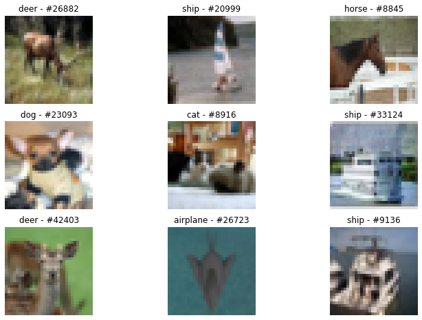
We also need a dictionary that would translate class numbers into their names, as defined by the CIFAR10 set, and a function to display a few randomly selected images.
# Translation between class id and nameclass_translator = { 0 : 'airplane', 1 : 'automobile', 2 : 'bird', 3 : 'cat', 4 : 'deer', 5 : 'dog', 6 : 'frog', 7 : 'horse', 8 : 'ship', 9 : 'truck',}
# Helper function printing 9 randomly selected pictures from the datasetdef print_images(): fig = plt.figure() fig.set_size_inches(fig.get_size_inches() * 2) for i in range(9): idx = torch.randint(0, 50000, (1,)).item() picture = detransformer(dataset[idx][0]) ax = plt.subplot(3, 3, i + 1) ax.set_title(class_translator[dataset[idx][1]] + ' - #' + str(idx)) ax.axis('off') plt.imshow(picture) plt.show()
Well, let’s take a look at a few elements of this dataset …
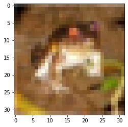
print(f'The first element of the dataset is a {class_translator[dataset[0][1]]}.')>>>The first element of the dataset is a frog.
image = detransformer(dataset[0][0])plt.imshow(image)
print_images()
Divide into training, testing and validation subsets
Note that the CIFAR10 dataset constructor allows us to retrieve either a training or a test subset. But what if we want to separate a validation subset that will allow us to determine the accuracy during training? We have to separate it out from the training dataset ourselves. The random_split function from the torch.utils.data package will be helpful here.
validation_length = 5000# Split training dataset between actual train and validation datasetstrain_dataset, validation_dataset = random_split(dataset, [(dataset_length - validation_length), validation_length])
Having three objects od the Dataset class: train_dataset, validation_dataset and test_dataset, we can define DataLoaders that will enable serving data in batches.
# Create DataLoaderstrain_dataloader = DataLoader(train_dataset, batch_size=batch_size, shuffle=True)validation_dataloader = DataLoader(validation_dataset, batch_size=batch_size, shuffle=False)test_dataloader = DataLoader(test_dataset, batch_size=batch_size, shuffle=False)
# Print some statisticsprint(f'Batch size: {batch_size} data points')print(f'Train dataset (# of batches): {len(train_dataloader)}')print(f'Validation dataset (# of batches): {len(validation_dataloader)}')print(f'Test dataset (# of batches): {len(test_dataloader)}')>>> Batch size: 256 data points>>> Train dataset (# of batches): 176>>> Validation dataset (# of batches): 20>>> Test dataset (# of batches): 40
Build a model
In order not to focus too much on the network architecture – as that is not the purpose of this post – we will use the network designed in this post on convolutional neural networks. It is worth noting, however, that one of the issues in network design is data dimensioning. To check the size of the input vector that will be served by a DataLoader, the following code can be run:
# Before CNN definition, let's check the sizing of input tensordata, label = next(iter(train_dataloader))print(data.size())print(label.size())>>> torch.Size([256, 3, 32, 32])>>> torch.Size([256])
So here we have a batch of size 256, then three RBG channels of the image, each with the size of 32 by 32.
This script can help in dimensioning a convolutional network. Of course, it is necessary to adapt it to the needs of a given model, but it’s a good start.
Eventually, our architecture will look like this:
class CifarNN(torch.nn.Module):
  def __init__(self):
    super().__init__()
    self.conv1 = Conv2d(3, 128, kernel_size= 5,5), stride=1, padding='same')  # [B, 128, 32, 32]
    self.bnorm1 = BatchNorm2d(128)
    self.conv2 = Conv2d(128, 128, kernel_size=(5,5), stride=1, padding='same')  # [B, 128, 32, 32]
    self.bnorm2 = BatchNorm2d(128)
    self.pool1 = MaxPool2d((2,2))  # [B, 128, 16, 16]
    self.conv3 = Conv2d(128, 64, kernel_size=(5,5), stride=1, padding='same')  # [B, 64, 16, 16]
    self.bnorm3 = BatchNorm2d(64)
    self.conv4 = Conv2d(64, 64, kernel_size=(5,5), stride=1, padding='same')  # [B, 64, 16, 16]
    self.bnorm4 = BatchNorm2d(64)
    self.pool2 = MaxPool2d((2,2))  # [B, 64, 8, 8]
    self.conv5 = Conv2d(64, 32, kernel_size=(5,5), stride=1, padding='same')  # [B, 32, 8, 8]
    self.bnorm5 = BatchNorm2d(32)
    self.conv6 = Conv2d(32, 32, kernel_size=(5,5), stride=1, padding='same')  # [B, 32, 8, 8]
    self.bnorm6 = BatchNorm2d(32)
    self.pool3 = MaxPool2d((2,2))  # [B, 32, 4, 4]
    self.conv7 = Conv2d(32, 16, kernel_size=(3,3), stride=1, padding='same')  # [B, 16, 4, 4]
    self.bnorm7 = BatchNorm2d(16)
    self.conv8 = Conv2d(16, 16, kernel_size=(3,3), stride=1, padding='same')  # [B, 16, 4, 4]
    self.bnorm8 = BatchNorm2d(16)
    self.linear1 = Linear(16*4*4, 32)
    self.drop1 = Dropout(0.15)
    self.linear2 = Linear(32, 16)
    self.drop2 = Dropout(0.05)
    self.linear3 = Linear(16, 10)
  def forward(self, x):
    # the first conv group
    x = self.bnorm1(self.conv1(x))
    x = self.bnorm2(self.conv2(x))
    x = self.pool1(x)
    # the second conv group
    x = self.bnorm3(self.conv3(x))
    x = self.bnorm4(self.conv4(x))
    x = self.pool2(x)
    # the third conv group
    x = self.bnorm5(self.conv5(x))
    x = self.bnorm6(self.conv6(x))
    x = self.pool3(x)
    # the fourth conv group (no maxpooling at the end)
    x = self.bnorm7(self.conv7(x))
    x = self.bnorm8(self.conv8(x))
    # flatten
    x = x.reshape( -1, 16*4*4)
    # the first linear layer with ReLU
    x = self.linear1(x)
    x = F.relu(x)
    # the first dropout
    x = self.drop1(x)
    # the second linear layer with ReLU
    x = self.linear2(x)
    x = F.relu(x)
    # the second dropout
    x = self.drop2(x)
    # the output layer logits (10 neurons)
    x = self.linear3(x)

    return x
Move to a GPU and calculate accuracy
Training a convnet on a CPU doesn’t make much sense. A simple test I did on the Google Colab showed that it takes around 2600 seconds to complete one epoch on a CPU, while on a GPU it took 66 seconds to do the same work. These times obviously depend on many factors beyond our control, such as what machines the Google Colab engine will direct us to, but the conclusions will always be similar – learning on a GPU can be much faster.
So what’s the easiest way to switch from CPU to GPU in PyTorch? Of course, in Google Colab we have to go through Runtime-> Change runtime type and change it to GPU. But the major changes need to be made in the code. Fortunately, there aren’t a lot of them, and they’re pretty straightforward.
The main issue is to establish what kind of environment we are dealing with. The code snippet below is a common good practice.
device = torch.device('cuda' if torch.cuda.is_available() else 'cpu')print(device)>>> cuda
In the next step, we create a model and move it to the currently available device.
model = CifarNN()model = model.to(device)
Before we start the training we need to define few parameters: number of epochs, learning_rate and optimizer, as well as what method will be used to calculate error. Here, there are also two lists, in which we are going to record accuracy for each epoch. This will allow us to draw a nice graph afterwards.
epochs = 40learning_rate = 0.001train_accuracies = [] # cumulated accuracies from training dataset for each epochval_accuracies = [] # cumulated accuracies from validation dataset for each epochoptimizer = Adam( model.parameters(), lr=learning_rate)criterion = CrossEntropyLoss()
The next code snippet is the main training loop. There are few things happening here that may be of interest to us in the context of this post, so I assigned indexes to some lines and commented them below:
(1) – we are going to measure time elapsed.
(2) – it is a good practice to signal to the PyTorch engine when a training takes place, and when we only evaluate on validation or test datasets. This significantly improves the performance of evaluation parts.
(3) – we move the data (batch) to a GPU.
(4) – values we get after passing the input through the network (here: yhat) are the so-called logits, i.e. values theoretically ranging from plus to minus infinity. Target on the other hand (here: y) contains the numbers 0 through 9 indicating a correct class. The function that calculates error (here: CrossEntropyLoss) internally handles the corresponding comparison of those values. However, when calculating accuracy – in point (5) – we must first calculate the network answer ourselves. We use the argmax function for this. It returns the index where the strongest (highest in value) network response occurs. This index will also be the number of the class to which the network assigned the input value. This way we get prediction – a vector containing the class assignment for each element of the currently processed batch.
(5) – the most convenient way to calculate accuracy based on data in two vectors: y and prediction is to use numpy – excellent for vectorized operations. In order for the data on a GPU to end up in the list processed in a CPU environment, we need to use .detach().cpu().numpy() command.
(6) – for each training epoch we process the validation subset and calculate its accuracy to compare it with the accuracy calculated for the training subset. This way we’ll see whether the training process is overfitting or not.
start = timer() # (1)for epoch in range(epochs): model.train() # (2) train_accuracy = [] for x, y in train_dataloader: x = x.to(device) # (3) y = y.to(device) # (3) optimizer.zero_grad() yhat = model.forward(x) loss = criterion(yhat, y) loss.backward() optimizer.step() prediction = torch.argmax(yhat, dim=1) # (4) train_accuracy.extend((y == prediction).detach().cpu().numpy()) # (5) train_accuracies.append(np.mean(train_accuracy)*100)
# for every epoch we do a validation step to asses accuracy and overfitting model.eval() # (2) with torch.no_grad(): # (2) val_accuracy = [] # accuracies for each batch of validation dataset for vx, vy in validation_dataloader: (6) vx = vx.to(device) # (3) vy = vy.to(device) # (3) yhat = model.forward(vx) prediction = torch.argmax(yhat, dim=1) (4) # to numpy in order to use next the vectorized np.mean val_accuracy.extend((vy == prediction).detach().cpu().numpy()) (5) val_accuracies.append(np.mean(val_accuracy)*100) # simple logging during training print(f'Epoch #{epoch+1}. Train accuracy: {np.mean(train_accuracy)*100:.2f}. \ Validation accuracy: {np.mean(val_accuracy)*100:.2f}') end = timer() # (1)
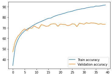
As a result of training on 40 epochs, we get the following metrics:
>>> Epoch #1. Train accuracy: 34.20. Validation accuracy: 47.32>>> Epoch #2. Train accuracy: 51.58. Validation accuracy: 57.00>>> Epoch #3. Train accuracy: 58.11. Validation accuracy: 61.56>>> Epoch #4. Train accuracy: 62.18. Validation accuracy: 64.16................................................................>>> Epoch #38. Train accuracy: 90.86. Validation accuracy: 73.86>>> Epoch #39. Train accuracy: 91.42. Validation accuracy: 73.30>>> Epoch #40. Train accuracy: 91.68. Validation accuracy: 73.40
As you can see, the difference between the training (91%) and the validation accuracy (73%) is considerable. The model fell into overfitting, which is visible on the graph below.
print(f'Processing time on a GPU: {end-start:.2f}s.') >>> Processing time on a GPU: 3113.36s.plt.plot(train_accuracies, label="Train accuracy")plt.plot(val_accuracies, label="Validation accuracy")leg = plt.legend(loc='lower right')plt.show()
The problem of overfitting is significant and there are several methods that can be used to reduce it. Some of them have been already applied to the above model (like the Dropout layer). More about preventing overfitting in this post.
At the end of the training process, we check how the model is doing on the test dataset, i.e. on the data that the model has never seen before.
# calculate accuracy on the test dataset that the model has never seen beforemodel.eval()with torch.no_grad(): test_accuracies = [] for x, y in test_dataloader: x = x.to(device) y = y.to(device) yhat = model.forward(x) prediction = torch.argmax(yhat, dim=1) test_accuracies.extend((prediction == y).detach().cpu().numpy()) # we store accuracy using numpy test_accuracy = np.mean(test_accuracies)*100 # to easily compute mean on boolean valuesprint(f'Accuracy on the test set: {test_accuracy:.2f}%') >>>Accuracy on the test set: 72.78%
Quick summary
This post was all about tools and techniques. We focused on few areas that are sometimes technically more difficult than the process of building the model architecture itself. We saw how to load data and divide it into three subsets: training, validation and test. We took a quick look at the transformations that can be applied using the transforms class and how one can display images from the dataset by inverting transformations. After a short stop at network dimensioning, our attention shifted to training in the GPU environment and calculating accuracy. The final accuracy of 72% on the test dataset obviously is not a premium result for the CIFAR10, but that was not the goal of the post. For those of you interested in increasing the accuracy and fighting overfitting, I recommend my post on data augmentation. BTW: the script used in this post is available in my github repo.