
Shape recognition, and handwritten digit recognition in particular, is one of the most graceful topics for anyone starting to learn AI. There are several reasons, but the two most important are the ease with which we can use well-prepared ready-made datasets and the ability to visualize these data.
From this tutorial you will learn:
- What is the MNIST dataset and what is the easiest way to load it for further use in the Keras library?
- How to visualize elements of the MNIST dataset?
- What is data normalization and how to normalize the MNIST dataset?
- How to build a simple model of a densely connected neural network using the Keras library?
- What is one-hot encoding?
- How to train a data classification model on the MNIST dataset?
- And how to assess the accuracy of the training process?
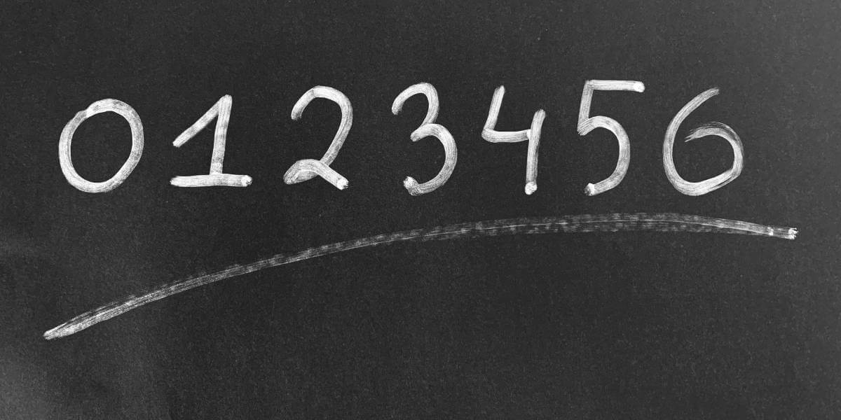
Okay, so without further delay let’s workshop on one of the simpler and better-known collections, the famous MNIST data set. The set consists of 60,000 elements in the training set and 10,000 in the test set. Each element is a 28 by 28 pixel image. The images are not colored, so for each pixel we have one value representing the shade of gray.
This is what the data sample in this set looks like. In the rest of the post, we’ll also look at individual data.

Are you an NBA fan? Check my free NBA Games Ranked service and enjoy watching good games only.
Handwritten digit recognition – importing and preprocessing data
At the very beginning pretty obvious move: we need to import the necessary libraries and data. We need the numpy library and of course Keras, which separates us from more complicated coding in TensorFlow. Note that we are also importing the MNIST file from keras.dataset. It is very convenient and will allow you to focus on the way you learn.
By the way: if you need to build a programming environment in which you’ll be able to carry out the work described in this post, you might want to read Development environment for machine learning.
import numpy as np import keras
>>> Using TensorFlow backend.
from keras.datasets import mnist
As seen above, keras used the Tensorflow library by default. If you prefer, you can use Theano for a change. By importing mnist we gain access to several functions, including load_data (). It downloads the MNIST file from the Internet, saves it in the user’s directory (for Windows OS in the /.keras/datasets sub-directory), and then returns two tuples from the numpy array.
(x_train, y_train), (x_test, y_test) = mnist.load_data()
>>> Downloading data from https://s3.amazonaws.com/img-datasets/mnist.npz
>>> 11493376/11490434 [==============================] - 5s 0us/step
The variable x_train contains images on which we will teach a neural network. We are dealing with a supervised learning, so for the network to learn, it must get information from us about what is in the picture. This information is in the variable y_train. We will call this data “labels”. The variable x_test contains pictures on which we will check whether the taught neural network can correctly recognize a digit that it has not seen before (on which it did not learn). To check if the neural network has correctly evaluated the content of the image, we must also have labels for the test set, which are located in the variable y_test. Ok, let’s see first what shape these variables have.
x_train.shape
>>> (60000, 28, 28)
x_test.shape
>>> (10000, 28, 28)
The training data contains, as expected, 60,000 elements, each with a size of 28 by 28 (pixels). The test data is 10,000. In both cases we are dealing with three-dimensional arrays, for which the first dimension is subsequent data samples (in total 60,000 and 10,000 respectively), and the next two dimensions store pixel values for each sample (for each image).
Displaying sample data
Let’s see one of the elements of the training set (x_train) and the label (y_train) assigned to it. For this purpose we will use the matplotlib.pyplot library, which we have to import first.
import matplotlib.pyplot as plt
%matplotlib inline
The <<% matplotlib inline>> command is specific to Jupyter Notebook and informs Jupyter that the results are to be displayed in the notebook window.
# Let's display 200 element from the training set and its label.
element = 200
plt.imshow(x_train[element])
plt.show()
# Let's display the label for this element
print("Label for the element", element,":", y_train[element])
>>> Label for the elementu 200 : 1
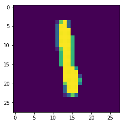
As you can see this is one. It is worth mentioning here that the MNIST dataset is not error-free. There are incorrect or doubtful classifications. For this reason, using even the most advanced teaching methods, it is not possible to achieve 100% correct classification in this relatively simple and well-defined set. For example, let’s take a look at element 500.
element = 500 plt.imshow(x_train[element]) plt.show() print("Label for the element", element,":", y_train[element])
>>> Label for the element 500 : 3
Is this three? Or maybe two? ;-). It’s hard to say.
Reshaping and normalizing
Quite an important issue: if we process an image in a neural network, it expects a vector and not a two-dimensional array. Unless the data first goes to a convolution, but that’s different story – a story about Convolutional Neural Networks, which will be covered in another post.
Therefore, before further processing, we should convert the training set to 60,000 x 784 (28 * 28). To change the shape of the data we will use the reshape function.
x_train = x_train.reshape((-1, 28*28))
The same of course for the test set, although instead of giving the formula 28 * 28 ,we give the target value immediately .
x_test = x_test.reshape((-1, 784))
Let’s check if the data has been transformed properly.
x_train.shape >>> (60000, 784)
x_test.shape >>> (10000, 784)
One of many good machine learning practices is data normalization. Before normalization, the value of each pixel – indicating the gray level of a given pixel – should be between 0 (typically 0 is completely black) and 255 (completely white). Everything in between is a shade of gray. Let’s check it:
print(x_train.min(), "-", x_train.max())
>>> 0 - 255
There are many ways to normalize data. The most common is zero-mean normalization, for which the new value W’ = (W – mean) / std. Subtracting the mean of the set and dividing by standard deviation. Such normalization is usually used when the minimum and the maximum values in the set are not specified. But we know what the minimum (0) and the maximum (255) values are, so we can apply “min-max” normalization. The formula for this normalization is quite extensive, although simple – I encourage you to search for it. However, for min = 0 and max = 255, we can simplify this formula significantly and simply divide the value of each pixel by the maximum value, i.e. 255.
x_train = x_train / 255 x_test = x_test / 255
Let’s check if, as expected, the maximum values will now oscillate between 0 and 1.
print(x_train.min(), "-", x_train.max()) >>> 0.0 - 1.0
Handwritten digit recognition – time for training
At this stage we have already prepared data for learning: x_train and y_train and for testing x_test and y_test. Time to teach and we’ll use the Keras library here. At the beginning we import the Sequential model, which you can read about here: https://keras.io/getting-started/sequential-model-guide/ and the import of two types of layers: Dense and Dropout.
Dense is a standard layer of the neural network in which each neuron is connected to each neuron of the next layer.
Dropout is a layer that prevents the phenomenon of over-fitting, i.e. over-matching the operation of the neural network to training data. If we deal with over-fitting, then after the training the network will get great results on the training set, and much worse on the test set (in general on data not previously seen). The Dropout layer in each learning cycle ignores a randomly selected group of neurons, which causes the network to generalize better.
Finally, we import the useful to_categorical() function, which we will use for one-hot encoding of labels – we’ll talk about that in a moment.
# creating model from keras.models import Sequential from keras.layers import Dense, Dropout from keras.utils import to_categorical
We create the model by entering any number of network layers in sequence. You can actually think of any architecture. I will limit myself to 4 Dense layers separated by a Dropout layer.
When creating a model, keep the following in mind:
- each layer has its activation function. Activation functions available in Keras are listed here: https://keras.io/activations/
- the last layer must have an activation function suitable for the task for which we built the network. If we are dealing with regression, i.e. a situation where the neural network is to predict the value (e.g. price of the house), then the activation function should be linear, because it should not process the network result in any way. If we are dealing with binary classification, i.e. we want the neural network to indicate whether we are dealing with class A or B (e.g. whether someone is at risk of lung cancer or not), then we will use the ‘sigmoid’ function. If we are dealing with a multi-class classification (e.g. classifying an image into one of 10 classes – as in our case), we will use the softmax function. Softmax will return a list of probabilities that an input sample belongs to a given class. For example, for the element 100 visualized above (which is class “one”), it can be the following vector: [0.02, 0.88, 0.003, 0.007, 0.01, 0.01, 0.035, 0.01, 0.005, 0.02] As you can see the highest probability will be on index 1, corresponding to the “one” class. Note that the probabilities naturally will add up to 1.0.
- Keras expects the first layer to be informed of the shape of the input vector. You can use the input_shape parameter, which expects a tuple consisting of the input vector dimension. For us, the vector is one-dimensional, hence 784 and None. The second method is to use the Dense layer parameter (other layers do not have it) input_dim = 784. The input vector dimension is given only for the first layer, because the size of the input vectors for subsequent ones will be calculated automatically based on the number of neurons in subsequent layers.
- each layer as the first argument takes the size of the output vector for the layer. As you can see from the model below, the first layer accepts 784 parameters and outputs 1024. The next one must naturally intakes 1024 (therefore for the next ones we do not have to specify the size of the input vector) and emits 128, etc.
- the number of layers and the size of the output vectors from each layer are arbitrary, but it should be remembered that the last layer must emit: 1 value for regression (because we predict one value) or n values for the n-class classification. For binary classification it will be 2. In our case, we have 10 classes, so it is a value of 10.
model = Sequential([ Dense(1024, activation='relu', input_shape=(784,)), Dense(128, activation='tanh'), Dropout(rate=0.05), Dense(64, activation='relu'), Dense(10, activation='softmax')])
After creating the model, we have to compile it. To do this, we call the method compile specifying:
- type of optimizer: https://keras.io/optimizers/
- loss function: https://keras.io/losses/
- and optional metrics that we want for our model to register. In our case we will use ‘accuracy’.
model.compile(
   optimizer='Adam',
   loss='categorical_crossentropy',
   metrics=['accuracy']
)
The last element of the learning process is calling the fit method, which implements the training of the neural network. At the entrance, we give the previously prepared training set (x_train), and because we are dealing with supervised learning, we also provide labels (y_train). It is good practice to shuffle the data, which reduces the risk of overfitting, hence shuffle = True.
In machine learning, a parameter often referred to as epochs appears – it specifies how many times the training set will be used in the learning process. Here, to teach a neural network, we will go through a training set 10 times, which means that the network will see 600,000 data samples in total.
Since most teaching methods do not use the Gradient Descent algorithm, but its computationally lighter Stochastic version, the batch_size parameter should also be provided, which determines how often we update the gradient. Gradient Descent is a topic for a separate post. We don’t necessarily want to deal with this right now :-). We need to explain this line of code, though:
y=to_categorical(y_train)
If we simply specify y = y_train in the fit method, Keras will report an error:
>>>Error when checking target: expected dense_4 to have shape (10,) but got array with shape (1,)
Where does it come from? As I wrote above, the last function in our network is softmax. Softmax will return a list of probabilities for the input data. For example, for the element 100 (the one visualized above) it could be the following vector:
[0.02, 0.88, 0.003, 0.007, 0.01, 0.01, 0.035, 0.01, 0.005, 0.02].
At the same time, in the hundredth element of the y_train table we have the value of 1. How would the neural network compare these two values and then calculate how far is it from the target (where the goal is to match a classification result with a label)? This cannot be done without transforming the target (labels) into so-called one-hot encoding. As a result, our “1” will be written in the following form:
[0.0, 1.0, 0.0, 0.0, 0.0, 0.0, 0.0, 0.0, 0.0, 0.0]
If we wanted to write the value 5 in this way, the vector would look like this:
[0.0, 0.0, 0.0, 0.0, 0.0, 1.0, 0.0, 0.0, 0.0, 0.0]
This operation of converting a scalar to a vector is performed by the function to_categorical().
OK, we’re ready to train the network.
model.fit(
   x=x_train,
   y=to_categorical(y_train),
   epochs=10,
   batch_size=64,
   shuffle=True
)
Model evaluation
The whole learning process took about 200s and we received accuracy of 99.42%. Since learning does not take long, you can try to play with the network – change the number of epochs, batch_size, type of optimizer or the structure of the network itself.
Of course, the accuracy indicated above was obtained on the training set. Now is the moment when we need the test set. The result on it will probably be slightly lower and if the difference will be greater than 2 – 4 percent, then we can risk the statement that we are dealing with overfitting and we need to change the model a bit.
To evaluate the effectiveness of the model, Keras gives us the evaluate method.
eval = model.evaluate(x_test, to_categorical(y_test))>>>10000/10000 [==============================] - 1s 100us/step
eval>>>[0.07423182931467309, 0.9811]
The result is assigned to the variable eval, which contains loss (here: 0.074) and accuracy of 98.11%. The difference between accuracy on the training and test set is only 1.31% and seems acceptable.
Keras offers us another interesting method, that can be used to predict values for new data (data that the network has not yet seen). Because we have not previously separated such a set, but only divided the MNIST set into learning and test data, we will just use a subset of the test data.
predictions = model.predict(x_test[0:100])
The method will return a 100-element scoreboard. Each element will indicate the probabilities that the input belongs to a given class. Let’s see what the prediction for x_test[0] looks like.
predictions[0]>>>array([3.7351333e-10, 2.8403690e-06, 3.6098727e-06, 2.9988249e-07,
1.5157393e-06, 5.1377755e-09, 1.6684153e-12, 9.9998987e-01,
1.9233731e-08, 1.7899656e-06], dtype=float32)
As you can see, most of the values are very small numbers (very low probability that the picture belongs to this class), except for the number at position 7 (counted from 0). Numpy has a very useful function that will save our eyes and immediately tell us which class was rated by the model as the most probable.
np.argmax(predictions[0]) >>>7
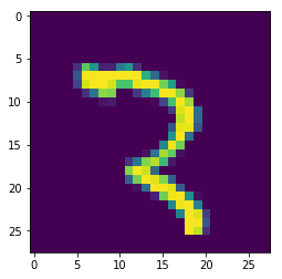
Let’s check what the picture looks like. Remember that the input data to the network were flattened for the purpose of learning to a vector with a length of 784. Before displaying it, we need to convert it back to the size of 28 x 28 pixels.
plt.imshow(x_test[0].reshape(28,28))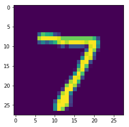
It looks nice, right? 🙂 OK, let’s see how all the predictions look after treating the probabilities with the argmax function. Note here: because we are dealing with a two-dimensional array, and not a vector as with the previous use of argmax, we must tell the function in what dimension it should analyze data. In our case, along the y axis, i.e. axis = 1.
np.argmax(predictions, axis=1)>>> array([7, 2, 1, 0, 4, 1, 4, 9, 6, 9, 0, 6, 9, 0, 1, 5, 9, 7, 3, 4, 9, 6, 6, 5, 4, 0, 7, 4, 0, 1, 3, 1, 3, 4, 7, 2, 7, 1, 2, 1, 1, 7, 4, 2, 3, 5, 1, 2, 4, 4, 6, 3, 5, 5, 6, 0, 4, 1, 9, 5, 7, 8, 9, 3, 7, 4, 6, 4, 3, 0, 7, 0, 2, 9, 1, 7, 3, 2, 9, 7, 7, 6, 2, 7, 8, 4, 7, 3, 6, 1, 3, 6, 9, 3, 1, 4, 1, 7, 6, 9])
Because the x_test [0: 100] set is not really new data and we have labels for them, we can display labels to compare the prediction with reality.
y_test[0:100]>>> array([7, 2, 1, 0, 4, 1, 4, 9, 5, 9, 0, 6, 9, 0, 1, 5, 9, 7, 3, 4, 9, 6, 6, 5, 4, 0, 7, 4, 0, 1, 3, 1, 3, 4, 7, 2, 7, 1, 2, 1, 1, 7, 4, 2, 3, 5, 1, 2, 4, 4, 6, 3, 5, 5, 6, 0, 4, 1, 9, 5, 7, 8, 9, 3, 7, 4, 6, 4, 3, 0, 7, 0, 2, 9, 1, 7, 3, 2, 9, 7, 7, 6, 2, 7, 8, 4, 7, 3, 6, 1, 3, 6, 9, 3, 1, 4, 1, 7, 6, 9], dtype=uint8)
At first glance, it looks basically the same. However, it is worth writing a neat formula that will calculate accuracy, because for 10 or even 50 data samples we can visually assess or calculate it manually, but for 1000 it definitely has not much sense 🙂
Let’s think what we compare with what? For sure, we compare the two formulas above, which leads us to:
np.argmax(predictions, axis=1) == y_test[0:100]>>>array([ True, True, True, True, True, True, True, True, False, True, True, True, True, True, True, True, True, True, True, True, True, True, True, True, True, True, True, True, True, True, True, True, True, True, True, True, True, True, True, True, True, True, True, True, True, True, True, True, True, True, True, True, True, True, True, True, True, True, True, True, True, True, True, True, True, True, True, True, True, True, True, True, True, True, True, True, True, True, True, True, True, True, True, True, True, True, True, True, True, True, True, True, True, True, True, True, True, True, True, True])
OK, this is not yet accuracy, but only an indication on which positions the predictions coincide with reality. To calculate accuracy, we will use Numpy and its mean function, which fortunately handles various types of data, including logical ones. The final formula:
np.mean(np.argmax(predictions, axis=1) == y_test[0:100])
>>> 0.99
The predictions of our network we’ve just trained for the first 100 test data have the 99% accuracy. I am tempted to check where the model was wrong, because apparently in one place it was wrong.
False is treated as 0 and True as 1. Fortunately, we have the argmin function, which also does well with logical data:
wrong_pred = np.argmin(np.argmax(predictions, axis=1) == y_test[0:100])
wrong_pred
>>> 8
element = wrong_pred
plt.imshow(x_test[element].reshape(28,28))
plt.show()
print("Label for the element", element,":", y_test[element])
print("Prediction for the element:", np.argmax(predictions[element]))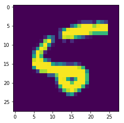
>>> Label for the element 8 : 5
>>> Prediction for the element: 6
As you can see the picture is marked as 5, and for the network it looks like 6. I admit that I’m not surprised. Probably it is actually five, strangely written, but if someone told me to say “quickly”, maybe I would bet on six.
If the learning lasted a long time, which probably does not happen in this case, it is worth saving the model using the save method.
model.save(r'<<insert-full-path-here-and-name-a-file-as-you-wish>>')
And that’s it. We’ve just built our first, simple handwritten digit recognition model – well done! 🙂
Was this post interesting and helpful to you? If so, please share it with your friends – thanks!
What other issues would you like to see on the blog? I encourage you to comment and ask questions.
Until next time 🙂
Are you an NBA fan? Check my free NBA Games Ranked service and enjoy watching good games only.