

Today I would like to present an example of using logistic regression and Keras for the binary classification. I know that this previous sentence does not sound very encouraging 😉 , so maybe let’s start from the basics.
We divide machine learning into supervised and unsupervised (and reinforced learning, but let’s skip this now). Supervised learning is one in which we teach a certain function to predict the result based on input data, having available pairs of examples: input data – result. It is like teaching a small child how different animals look, by repeatedly showing pictures and explaining: “… here’s a dog, here is a horse, again it’s a dog …”. On the other hand, unsupervised learning uses information that is not classified, i.e. it does not have specific categories (results). The goal of unsupervised learning can be, for example, dividing a data set into categories based on the similarities and differences that the algorithm will automatically capture in the set. For example, you could try to group photos of animals into two classes: land and sea. A suitable machine learning algorithm or neural network could separate them into such two groups based on the captured animal traits (e.g. fins vs legs).
For the purposes of this post, let’s focus more on a supervised learning. It contains two categories of tasks: regression and classification. Regression tries to predict a numerical (continuous) value, e.g. real estate value or share price. Classification designates categories based on the input data. For example, based on a picture with a handwritten number, it specifies what number it is.
Logistic regression is a supervised learning, but contrary to its name, it is not a regression, but a classification method. It assumes that the data can be classified (separated) by a line or an n-dimensional plane, i.e. it is a linear model. In other words, the classification is done by calculating the value of the first degree polynomial of the following form:
y =ω1*x1+ω2*x2+…+ωn*xn
where x is the input parameter, ω is the weight assigned to this parameter, and n is the number of input parameters. The next step in logistic regression is to pass the so obtained y result through a logistic function (e.g. sigmoid or hyperbolic tangent) to obtain a value in the range (0; 1). After obtaining this value, we can classify the input data to group A or group B on the basis of a simple rule: if y > = 0.5 then class A, otherwise class B.
Machine learning process is based on choosing the weights ω in such a way to get the highest percentage of correct classifications on a training set. This is achieved by calculating the error function and its minimization (i.e. error minimization) using a gradient descent algorithm.
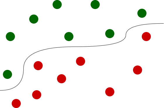
Simple example: let’s assume that our data that we have prepared for learning looks like this:

It is quite easy to see that we are dealing here with two types of “dots”: green and red. What’s more, the data looks easily separable by a line and in the learning process, using logistic regression for example, you can teach the machine to separate these classes. Linear function separating the classes could look like this:
Having trained classifier, we could classify new data that the machine have not seen before. They could look for example like this:

Trained classifier accepts parameters of new points and classifies them by assigning them values (0; 0.5), which means the “red” class or the values [0.5; 1) for the “green” class.
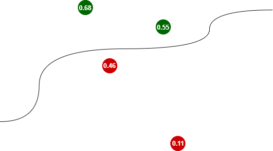
Note that the further from the separating line, the more sure the classifier is. For the farther away red dot the value is closer to zero (0.11), for the green one to the value of one (0.68).
It may sound quite complicated, but the available libraries, including Keras, Tensorflow, Theano and scikit-learn do most of the hard work for us, including all calculations. I hope to write a post about logistic regression soon, where I will explain this issue a bit better, also from the mathematical point of view, but at the moment the above information should be enough to build a simple classifier.
The most commonly used type of logistic regression is a binary logistic regression, when we classify the input data into one of two categories (hence the binary). And this is the issue we will address in this post. We will use the MNIST set, which I wrote more about in this post.
However, the MNIST data set has 10 classes, so we will have to limit it to two, which itself is an interesting programming exercise.
OK, enough of this theoretical introduction, let’s get to work! 😎
If you need to build a programming environment in which you’ll be able to carry out the work described in this post, I invite you to read the post Development environment for machine learning.
Are you an NBA fan? Check my free NBA Games Ranked service and enjoy watching good games only.
Logistic regression and Keras – coding
To begin with, we import numpy and the Keras library and display its version.
import numpy as npfrom tensorflow import kerasprint (keras.__version__)
>>> 2.2.4-tf
We import MNIST data set directly from the Keras library. If you need more information about the MNIST data set, take a look at this post.
from keras.datasets import mnist
We import data into variables and check their shape.
(x_train, y_train), (x_test, y_test) = mnist.load_data()x_train.shape>>> (60000, 28, 28)y_train.shape>>> (60000,)
Let’s check the first 10 labels.
y_train[0:10]>>> array([5, 0, 4, 1, 9, 2, 1, 3, 1, 4], dtype=uint8)
As you can see they contain different digits. And we are only interested in any two of them, because we want to carry out binary classification, i.e. division into two sets. We’ll take care of ones and zeros, but you can choose any pair of digits. Using a small programming trick, we create new variables that contain only zeros and ones.
x_train_new, y_train_new = x_train[(y_train==0) | (y_train==1)], y_train[(y_train==0) | (y_train==1)]
Let’s check the shape of the new variables.
x_train_new.shape>>> (12665, 28, 28)y_train_new.shape>>> (12665,)
As you can see, we have a subset of 12665 elements (only zeros and ones) selected from the full set, which contains 60,000 elements (all digits). To make sure we only have zeros and ones, we’ll display the first 10 labels again.
y_train_new[0:10]>>> array([0, 1, 1, 1, 1, 0, 1, 1, 0, 0], dtype=uint8)
It’s good! 🙂 The MNIST data set provides data in the form of images with a resolution of 28 x 28 pixels. Consequently, the variable x_train_new is a three-dimensional array of data in which the first dimension is the index of the set and the other two dimensions contain data for each image. For machine learning purposes, however, we need to flatten data into two dimensions only: index and flattened image data (28 * 28 = 784).
x_train_final = x_train_new.reshape((-1, 784))x_train_final.shape>>> (12665, 784)
A similar sequence of operations we perform for the test set.
x_test_new, y_test_new = x_test[(y_test==0) | (y_test==1)], y_test[(y_test==0) | (y_test==1)]x_test_new.shape>>> (2115, 28, 28)x_test_final = x_test_new.reshape((-1, 784))
The last element of data preprocessing is their normalization.
x_train_final = x_train_final / 255x_test_final = x_test_final / 255
Having the data in the four final variables: x_train_final, y_train_new, x_test_final and y_test_new, we can proceed with creating the model. We use the keras.Sequential model and we define one layer only, that will take an image at the input, calculate the polynomial value: x1 * w1 + x2 * w2 + … + x784 * w784, and then pass the result through the sigmoid function that will squeeze it into a range (0; 1).
model = keras.Sequential({ keras.layers.Dense(1, input_shape=(784,), activation='sigmoid')})
In the next step, Keras expects the model to be compiled by calling the compile method. This step specifies:
- type of optimizer: we use the stochastic gradient descent
- loss function: Keras offers many different loss functions: http://keras.io/losses. In our case binary_crossentropy will be the most appropriate function
- optionally, you can define a metric that will track training progress
model.compile(optimizer='sgd', loss='binary_crossentropy', metrics=['binary_accuracy'])
The model is now ready for training. To start it, we call the fit() method, passing the following data:
- training data set, including labels
- number of epochs, which indicates how many times the training set is going to be used in the training process – here we will process it 5 times. You can easily change this parameter to experiment, but it won’t have much effect on the final result. In the sense that even setting it to 1 can give relatively good results, and setting it to a high value will not significantly improve the result, and will certainly lengthen the calculation and can lead to over-fitting
- whether to shuffle the data before moving on to the next epoch (strongly recommended)
- and the batch_size. This parameter determines how many data samples are used to calculate gradient updates. Processing in batches significantly speeds up the calculations, because the gradient is calculated only for the given batch, not for the whole set.
model.fit( x=x_train_final, y=y_train_new, shuffle=True, epochs=5, batch_size=16)
>>> Epoch 1/5
>>> 12665/12665 [==============================] - 1s 93us/sample - loss: 0.0828 - binary_accuracy: 0.9853
>>> Epoch 2/5
>>> 12665/12665 [==============================] - 1s 92us/sample - loss: 0.0213 - binary_accuracy: 0.9972
>>> Epoch 3/5
>>> 12665/12665 [==============================] - 1s 96us/sample - loss: 0.0154 - binary_accuracy: 0.9975
>>> Epoch 4/5
>>> 12665/12665 [==============================] - 1s 95us/sample - loss: 0.0127 - binary_accuracy: 0.9976
>>> Epoch 5/5
>>> 12665/12665 [==============================] - 1s 76us/sample - loss: 0.0111 - binary_accuracy: 0.9977
Already after the first epoch the accuracy reaches 98.5%. We have 99.77% after five epochs. However, the real test for the algorithm is, of course, the verification on a set that the algorithm has not seen before. In our case, it will be the x_test_final set and its labels y_test_new.
eval = model.evaluate(x=x_test_final, y=y_test_new)>>> 2115/2115 [==============================] - 0s 51us/sample - loss: 0.0065 - binary_accuracy: 0.9995
eval
>>> [0.006539232165791561, 0.9995272]
Interestingly, we have obtained even better result – 99.95%. Let’s save the model to a file.
model.save(r'./logisticRegressionKeras.hdf5')
Are you ready for more? Great! 😎
Since we have saved the model to a file, it can be used in any other notebook. Below I will show how this can be done, and we’ll also do a small, you might say home experiment 😉 with trying to recognize my handwriting. But let’s start with the necessary imports (remember that I assume work in a new notebook, so imports are necessary).
import numpy as npfrom tensorflow import kerasfrom PIL import Imagefrom matplotlib.pyplot import imshow%matplotlib inline
We load the model from the file into the model variable using the load_model () function.
model = keras.models.load_model(r'./logisticRegressionKeras.hdf5')
To start with, let’s check if our model still works and correctly classifies the test set. For this purpose, we load the MNIST data set, from which we are only interested in the test data. Again, we only choose zeros and ones, because our model can only recognize these two digits. We change the shape of the data and normalize it, and then call the model.evaluate () method.
from keras.datasets import mnist
(x_train, y_train), (x_test, y_test) = mnist.load_data()x_test_new, y_test_new = x_test[(y_test==0) | (y_test==1)], y_test[(y_test==0) | (y_test==1)]
x_test_final = x_test_new.reshape((-1, 784)) / 255
eval = model.evaluate(x=x_test_final, y=y_test_new)>>> 2115/2115 [==============================] - 0s 22us/sample - loss: 0.0065 - binary_accuracy: 0.9995eval>>> [0.006539232165791561, 0.9995272]
It seems that the model has successfully loaded and gives the correct results on the set of ones and zeros from MNIST.
What if we did a small experiment on non-MNIST data? I thought that I would create pictures with “handwritten” zeros and ones, I would process them into a form similar to the data from the MNIST set and see what the model would say. I deliberately used quotation marks (“handwritten”), because I drew them with the mouse in Paint, previously setting the size of the image to 28 x 28 pixels. I saved the images as a bitmap on the disk. The files obtained in this way require loading into the numpy array and a gray scale conversion – see the first line of code of the following convert_image() function (for both tasks I needed the PIL library imported above).
Unfortunately, conversion using the convert(‘L’) method gives an inverted gray scale. I.e. in places where the value of pixel brightness should be 0 we have 1 and vice versa. Hence, I had to subtract 1 and multiply by (-1). In addition, as a result I received “negative zeros” (values shown as -0.). Hence for certainty the function abs () was used – see the second line of the convert_image () function. I encourage you to repeat my experiment and draw your numbers by yourself.
def convert_image(file): image = np.array(Image.open(file).convert('L')) return np.abs(((image / 255) - 1)*(-1))
Let’s see what my zero looks like and whether it is correctly classified.
im = convert_image(r'<<insert-full-path-here>>/moje-zero.bmp')imshow(im)

predict_input = im.reshape((-1,784))prediction = model.predict(predict_input)prediction>>> array([[0.00267569]], dtype=float32)
The classification result (0.0027) is close to 0.0, which means “zero” for my classifier.Great!
And what result will we get for my “handwritten one”?
im = convert_image(r'<<insert-full-path-here>>/my-one.bmp')imshow(im)

predict_input = im.reshape((-1,784))prediction = model.predict(predict_input)prediction>>> array([[0.9701028]], dtype=float32)
We have 0.97 here, so quite a certain classification as “one”. So it seems that the classifier built on the basis of logistic regression was able to generalize the problem quite well and also works outside the MNIST set. Of which I am very happy 🙂 .
If someone would like to experiment on their own, then a nice idea seems to be choosing two other digits from the MNIST set and checking if similar results can be obtained. It may also be interesting to draw your own handwritten numbers. Or maybe a change in the logistics function to tanh?
Did you like this post about logistic regression and Keras? If so, please recommend it to people you know who might be interested in the topic – thanks!
What other issues would you like to see on the blog? I encourage you to comment and ask questions.
Would like to read more about machine learning? Try my other posts: Naive Bayes in machine learning or Handwrittien Digit Recognition with Python and Keras.
Until next time!
Are you an NBA fan? Check my free NBA Games Ranked service and enjoy watching good games only.
Why the dense unit is 1? Shouldn’t it be 10 since we have 0-9 output digits?
First of all, you’re right that in the MNIST dataset we have digits from 0 to 9. However, in this exercise I wanted to perform binary classification, which means choosing between two classes. I chose 0s and 1s and eliminated other digits from the MNIST dataset.
Then, as for this line of code: keras.layers.Dense(1, input_shape=(784,), activation=’sigmoid’). I used Dense layer to get input vector of 784 data points and squeeze it to a range (0;1) using sigmoid and then output one value only. The first parameter of Dense method is described as “dimensionality of the output space” – in our case is a single number, hence we have “Dense(1, …)”.
You may also wonder why we use Dense layer for logistic regression. Well, while performing a logistic regression we want to first calculate the polynomial value of: x1 * w1 + x2 * w2 + … + x784 * w784 and this is exactly what Dense layer does.
why I choose the 1s and 2s or other digits, the accuracy will be like 0.17 and some are much more lower.
model = keras.Sequential({
keras.layers.Dense(1, input_shape=(784,), activation=’sigmoid’)
})
doesn’t work. gives several errors. like “The added layer must be an instance of class Layer.” or later “TypeError: add() missing 1 required positional argument: ‘layer'” and after that “‘NoneType’ object has no attribute ‘compile'”
Hi, you probably use a newer version of Keras. From 2.2.4 import was changed for layers. Try tensorflow.keras.layers instead. Also: https://stackoverflow.com/questions/55324762/the-added-layer-must-be-an-instance-of-class-layer-found-tensorflow-python-ke