

At the time of writing this post (its Polish version was created in April/May 2023), there’s still quite a widespread excitement about the possibilities of large language models. These possibilities were spectacularly showcased to us by a solution released at the end of 2022 by OpenAI, and our world will never be the same again. Large language models, including conversational ones like ChatGPT, mostly use variations of the Transformer architecture. A landmark in this area is the groundbreaking paper by Google engineers in 2017: “Attention is all you need“1, which proposed the use of an encoder-decoder architecture variant, combined with the so-called self-attention mechanism and a few clever tricks, to build a model that would effectively translate from one language to another. This model was named Transformer and even though it didn’t seem groundbreaking at first, it stormed not only the NLP domain but also image processing within a few years. In this blog post, I’d like to show how you can build a small language model based on this concept, trained on 19th-century classic Polish literature, that can be used to generate texts reminiscent of the original source. For English-speaking readers, the choice of Polish literature may not be the best, but it is quite easy to replace the Polish source text with any English one. e.g. the works of William Shakespeare.
The post was mainly based on my experiments with coding relatively simple language models. It’s based on part of the Transformer architecture (the model is decoder-based) and inspired by a series of tutorials by Andrej Karpathy2. It is aimed at people who already have some basic knowledge of NLP and a toolset that includes Python and the Pytorch library. It’s hardly possible to fit everything that should be written about into one post. Therefore, I plan to create three parts and eventually something like a small tutorial, that will encourage you to write part of the code by yourself. By the way: there is another, in my highly subjective opinion 😉 quite good, tutorial about convolutional neural networks available on this blog. If anyone wants to know CNNs from the inside out, here is the first part of that tutorial.
Summing up, in the first part:
- we will take a bird’s eye view of the classic Transformer architecture and determine what parts we can pick for ourselves,
- we will create a class implementing a feed forward neural network – this class will then be used to build the model,
- we will make a simple implementation of the self-attention mechanism, and also discuss why and how we mask the future in the decoder,
- we will create a class implementing masked self-attention. We will use this class later when building our text generator.
In the second part:
- we will implement a class performing multi-head masked self-attention,
- we will prepare a training set for the model,
- we will focus our attention for a moment on character/word embedding and how this translates to our model,
- we will build the main class of the model to put everything together.
The third part includes:
- creating the main learning loop,
- adding validation and saving the model to a file,
- training the model in Google Colab,
- using the trained model to generate some probably a gibberish text.
The last issue: the code will be embedded in the content but also available on GitHub. However, I will write this post in such a way that it is worth trying to implement the code by yourself. I know from myown experience that creating a code to implement someone else’s idea is not an easy task, but the time spent on an independent (even if ultimately not entirely successful) coding will pay off in the future. You can use Google Colab or any other environment for implementation, preferably with a GPU available.
Transformer architecture
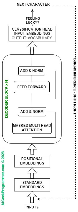
Let’s look at the Transformer architecture and think about what we can take from it to achieve our goal. From a bird’s eye view, the classic Transformer consists of two elements: an encoder and a decoder. The encoder takes the text to be translated, generates an internal representation from it (named “encoded features” in Figure 1) using the self-attention mechanism and a neural network, and passes it to the decoder. The decoder receives input from the encoder and, being an autoregressive model, also consumes the output of its previous step. Hence, in the figure, you can see that the decoder’s input also includes the result of the translation “shifted to the right”. This sometimes doubtful “shifted right” simply means that when predicting a token at step T, the decoder takes the translation state from step T-1 as input.
Both the encoder and the decoder consist of N sub-blocks. The number N is arbitrary here so the number of sub-blocks can vary. In the original paper, N was set to 6. The sub-blocks in the encoder and decoder differ slightly from each other, which is best seen in figure 2:
So, what do we have in this architecture…
a) The most interesting element is the Multi-Head (Self) Attention (1). We’ll take a closer look at it in a moment. Generally, self-attention enables identification of dependencies between words in the sentence being translated. This was something that Recurrent Neural Networks did well, but due to the sequential processing of data in RNNs, in practice they were not feasible for use on very large datasets. The Self-Attention module has the ability to process data highly parallel and relies on mass matrix multiplications, which GPUs are built for. It is worth noting that Multi-Head Attention has a somewhat more complex “sister” in this architecture, the Masked Multi-Head Attention (4). Why and how we mask in the decoder will be explained later in the post.
b) In the diagram, we have an Add & Norm (2) element in several places. Add refers to the so-called skip-connection. Information flows forward through this connection, bypassing the self-attention block, and the gradient freely flows back during the optimization process. Norm refers to the Layer Normalization (LN), which normalizes all input data within one vector, so normalization is performed horizontally. It’s worth noting here that LN works differently than Batch Normalization (BN). BN normalizes one input variable along the entire data batch, so vertically. If someone wanted to better understand this, here is a good explanation of the differences between LN and BN. Pytorch offers an implementation of LN, so adding it to the model will be relatively easy.
c) Next on the diagram, we find a standard densely connected neural network, described as “Feed Forward” (3). After exiting the decoder, we have a linear transformation (8), which simply changes the decoder’s output signal to the expected size. This size is the size of our model’s dictionary, because ultimately the model generates a probability distribution from which we can extract the most likely next word or part of a word. Yes! Ultimately, all language models, even the largest ones with hundreds of billions of parameters, generate a probability distribution on output, from which you can extract the most likely next word or group of most likely words. By the way, I wonder if our brain, when we’re talking, also tries to predict the most likely next word? Hmmm… 😉
d) The last part of the model is the input data. A string of words (e.g., a sentence to be translated) is fed into the encoder. What is done here is called word embedding, which transforms each word (or part of a word, because not always whole words become tokens – it depends on the type of embedding used) into its digital representation (5). Then information about the positions of words in the sentence is added – “Positional Encoding” (7). This is significant for the model for two reasons. First, in the case of a model translating between languages, information about the order of words in language A is significant for generating the translation in language B, because languages usually have different syntactic structures (different parts of speech occur in different places). The second reason is that, unlike the RNNs, the Transformer is not a sequential model. A sequential model processes consecutive words, so it implicitly “knows” their order. In the case when we throw the whole sentence into the Transformer at once in the form of a matrix and process it in parallel through all elements of the model, this information is lost and must be replaced somehow. This role is performed by Positional Encoding.
e) The decoder also receives Positional Encoding (7) and the translation state from moment T-1, i.e., it consumes its output – so it is an autoregressive model. The output is also embedded by the same mechanism we use in the encoder (6). I wrote a few paragraphs above about why the input to the decoder is marked as “Outputs – shifted right”.
Let’s cherry-pick the best parts…
Well, okay, we might not want any other architecture than Transformer, but do we need its entirety for our task? The original Transformer architecture was used for translation. We do not want to make translation. We want to generate text. The decoder deals with generating after we have previously taught the model the structure of our language. Hence, to continue, we will discard the whole encoder from our little model and stay with the decoder only. Additionally, since we don’t have data from the encoder, the middle element, marked on Figure 2 with number 1, i.e., multi-head attention, will also be dropped from the decoder. The model architecture for this tutorial will ultimately look like this.
So we have a few elements to build here. Let’s start with the simplest one – the “Feed Forward”. This is an implementation of a simple multi-layer perceptron, with one hidden layer. If you program in Pytorch, I suggest you try writing a class yourself, let’s call it “FFNN”, inheriting from nn.Module, which will take the following input parameters: input layer size (input_dim), hidden layer size (hidden_dim), and output layer size (output_dim). It will then perform a linear transformation – nn.Linear() – from the input to the hidden layer and from the hidden to the output layer. Let’s take relu() as the activation function, and before returning the result, let’s add a dropout layer for regularization. Of course, Pytorch convention requires that, besides the init() constructor, the class implements a forward() method. You can compare the result of your work with the code below.
import torch
import torch.nn as nn
import torch.nn.functional as F

# class for FFNN
class FFNN(nn.Module):
    def __init__(self, input_dim, hidden_dim, output_dim):
        super().__init__()
        self.fc1 = nn.Linear(input_dim, hidden_dim)
        self.fc2 = nn.Linear(hidden_dim, output_dim)
        self.dropout = nn.Dropout(0.1)

    def forward(self, x):
        x = self.fc1(x)
        x = F.relu(x)
        x = self.fc2(x)
        x = self.dropout(x)
        return x
The next element is the masked multi-head (self) attention. However, before we create a class to handle this element, let’s look at the self-attention mechanism on a simple example. The mechanism of the biological attention, i.e., focusing on the relevant thing at the moment, is an elementary cognitive process in humans. It has been transferred to the NLP domain and in general to machine learning, so that the model can focus its attention on elements that are significantly related to each other in a sentence. In the already quoted study “Attention Is All You Need”, the authors show the operation of the attention mechanism in the sentence “a majority of American governments have passed new laws since 2009 making the registration of voting process more difficult.”
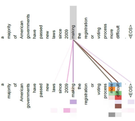
The attention calculated for the word “making” shows that the mechanism was able to catch quite distant but obviously significant dependencies between the word “making” and “more” and “difficult”. In the picture, the intensity of the color of the connecting line corresponds to the intensity of attention between the word “making” and the other words in the task. Do you still remember Recurrent Neural Networks? Me neither ;-). One of the features of RNNs was that they processed words / tokens sequentially, one after another. While processing the next word in the sentence, they take into account the state of the network for the previous token. In this way, dependencies between words in a sentence are identified. With the drawback that these dependencies would become weaker as you move away from the word “making”. Some of the RNN problems were solved by using LSTMs and GRUs, but practice shows that the self-attention mechanism is a much more effective solution. Dependencies between words in a sentence are important not only for translation models, but generally for all language models. They allow the model to “understand” the language structure. From this perspective, the self-attention mechanism becomes a key element of any language model.
Now that we know what self-attention is for, let’s see how it works. At the input, as is often the case in machine learning, the mechanism receives a matrix of data. Each row of this matrix is a “word”. For our example, let’s assume that we are processing 10 words at the same time. Put simply, let’s assume that the length of the longest sentence is equal to 10 words. In practice, these values are of course much larger.
Here’s a small digression: the ability to process a large amount of information in parallel is the main advantage of the Transformer architecture over RNN, which as I mentioned earlier, processes information sequentially and therefore much slower. In other words, in the Transformer architecture, everything happens as it should, i.e., on the principle of multiplying large matrices – and this operation is very much liked by GPUs.
OK, so the matrix has 10 rows, each row contains a “word” transformed into a digital representation in the embedding process (standard and positional embeddings). For simplicity, let’s assume that the embedding dimension is 32. It can be arbitrary, but in the original architecture various values were experimented with: 128, 256, 512, finally settling on the latter.
import torch

# We have an input vector X of 10 tokens (rows), each token embedded in 32 dimensions (columns)
X = torch.randn(10, 32)
In the process of calculating attention, we define three matrices of model parameters: Query, Key, and Value. These matrices contain model parameters, which means that during training, the values of these matrices are learned to optimal values:
# Query parameters matrix Q is 32x32
pQ = torch.randn(32, 32)

# Key parameters matrix K is 32x32
pK = torch.randn(32, 32)

# Value parameters matrix V is 32x32
pV = torch.randn(32, 32)
The number of rows in these matrices is the same as the number of columns in X (otherwise, the multiplication would fail). The number of columns is the same as the number of rows in order to maintain the input size.
In the first step, we multiply the input matrix X by each of the three parameter matrices:
# step 1 of attention: multiply parametric query matrix pQ with X
# pQ is 32x32, X is 10x32, so the result is 10x32
Q = torch.matmul(X, pQ)

# step 2 of attention: multiply parametric key matrix pK with X
# pK is 32x32, X is 10x32, so the result is 10x32
K = torch.matmul(X, pK)

# step 3 of attention: multiply parametric value matrix pV with X
# pV is 32x32, X is 10x32, so the result is 10x32
V = torch.matmul(X, pV)
As a result, we get three Query, Key, and Value matrices (Q, K, V), on which we perform the following operation:
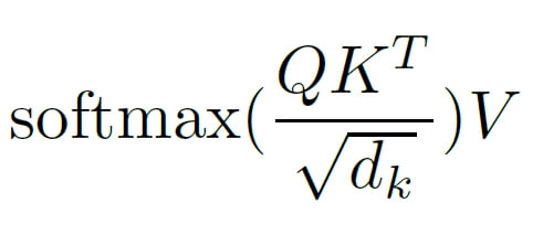
What actually happened here? In the numerator, we multiply the Query matrix by the transposed Key matrix. Since the size of Query is 10×32 and the size of the transposed Key is 32×10 (we swapped columns with rows), the resulting QKT matrix will have a size of 10×10. What does it contain? The result can be understood as an answer to the question “How important is the key for the query?”. In other words, we get weights that indicate which words in the analyzed sentence may be significant for each other. Of course, this information will become actually valuable after training the model, i.e. after optimizing the weights in the Query and Key matrices.
The operation of dividing by the square root of the key dimension dk (see denominator) is intended to scale the result to eliminate potentially large matrix product values. This is important because we later perform the softmax operation, which can become numerically unstable for large values (very large values or NaN may appear). After executing the softmax function, we get a 10×10 matrix, which contains a normalized score indicating mutually significant word connections in a given sentence. In the last step, we multiply this score by the V matrix of size 10×32, obtaining an output of self-attention of size 10 x 32, the same as the input X. Here’s how it might look in code, on a simple example:
# step 4 of attention: calculate the attention weights
# Q is 10x32, K is 10x32, so the result is 10x10
# we need to transpose K to make it 32x10
# we need to divide by sqrt(32) to normalize the weights
weights = torch.matmul(Q, torch.transpose(K, 0, 1)) / torch.sqrt(torch.tensor(32))

# step 5 of attention: apply softmax to the weights
# weights is 10x10, so the result is 10x10
weights = torch.softmax(weights, dim=1)

# step 6 of attention: multiply the weights with the values
# weights is 10x10, V is 10x32, so the result is 10x32
output = torch.matmul(weights, V)
These operations ensure that as the model gradually learns and optimizes the values of its parameters pQ, pK, and pV, it increasingly accurately detects and maps the connections between words in a sentence. And these connections are essential for performing translation or generating new text. The attention mechanism can also be viewed through the prism of analogy to Convolutional Neural Networks, in which we have a convolution operation performed using filters. Filters are also matrices with model parameters and are also learned (optimized) to detect important features of the analyzed image as accurately as possible.
Oh no! Not the masking again!
We still need to discuss the topic of masking. There are two types of masking in the Transformer architecture: padding and look-ahead. Although we won’t be using padding in our solution, it’s still worth dedicating some time to this topic. Let’s assume that we’re embedding each token in a 4-dimensional space. That means each token will be represented as a vector with 4 numbers and we’ve set a maximum sentence length of 5 tokens for our model. Of course, these are not realistic values, but they simplify the analysis. Now, let’s assume that we have 2 sentences in our training set or batch:
“to be” and “or not to be”
First, we turn each sentence into tokens. We want each sentence to be the same size before we feed it to our model – in our case, 5 tokens. In instances where we lack words to reach this maximum size, we fill in the gaps with a special token <pad>. After tokenization, our sentences look like this:
["to", "be", <pad>, <pad>, <pad>] and ["or", "not", "to", "be", <pad>]Next, we assign each token a numerical representation, where our special token is given the value zero – the numbers below are arbitrary and created purely for this example.
[[ 0.1, -0.2,  0.3, 0.5], # "to"
[  0.4,  0.6, -0.1, 0.2], # "be"
[  0.0,  0.0,  0.0, 0.0], # <pad>
[  0.0,  0.0,  0.0, 0.0], # <pad>
[  0.0,  0.0,  0.0, 0.0], # <pad>
[  0.1, -0.2,  0.3, 0.5], # "or"
[  0.4,  0.6, -0.1, 0.2], # "not"
[  0.1, -0.2,  0.3, 0.5], # "to"
[  0.4,  0.6, -0.1, 0.2], # "be"
[  0.0,  0.0,  0.0, 0.0]] # <pad>
How many of these paddings will there be in the input? In the original article Vaswani et. al did not provide a single value for maximum sentence length, but experimented with values such as 60 and 128. So there can be a lot of them, and their primary use is to allow the model to process sentences of different lengths, which they do perfectly well. Do we want the model to learn these <pad> tokens though? For obvious reasons, no. They are merely a technical addition and the model should simply ignore them. Ignoring is done by masking the padding. Creating a mask can be done, for example, in this way:
input_tensor = torch.tensor(
                [[0.1, -0.2,  0.3,  0.5],  # "to"
                 [0.4,  0.6, -0.1,  0.2],  # "be"
                 [0.0,  0.0,  0.0,  0.0],  # <pad>
                 [0.0,  0.0,  0.0,  0.0],  # <pad>
                 [0.0,  0.0,  0.0,  0.0],  # <pad>
                 [0.1, -0.2,  0.3,  0.5],  # "or"
                 [0.4,  0.6, -0.1,  0.2],  # "not"
                 [0.1, -0.2,  0.3,  0.5],  # "to"
                 [0.4,  0.6, -0.1,  0.2],  # "be"
                 [0.0,  0.0,  0.0,  0.0]]) # <pad>
# Please note that <pad> token is always 0.

# Create a boolean mask of the same shape as the input tensor, where True indicates a padding token
padding_mask = input_tensor.eq(0.0)
print(padding_mask)

> tensor([[False, False, False, False],
>         [False, False, False, False],
>         [ True,  True,  True,  True],
>         [ True,  True,  True,  True],
>         [ True,  True,  True,  True],
>         [False, False, False, False],
>         [False, False, False, False],
>         [False, False, False, False],
>         [False, False, False, False],
>         [ True,  True,  True,  True]])
We, however, are more interested in look-ahead masking, which occurs in the decoder during the multi-head masked self-attention operation. I’d like to highlight a key difference between padding masking and look-ahead masking. The former is performed on the model input, while the latter is performed on the self-attention weight matrix. This distinction is worth emphasizing as it may not be apparent at first glance.
Why do we mask self-attention in the decoder? We want to enforce that the self-attention mechanism focuses solely on the current and past tokens, ignoring any associations with future tokens. Otherwise, we would train the entire mechanism to peek into the future. While this future peeking would be theoretically possible during the training phase, what could it peek into when it is supposed to generate this future itself, during the operation of a trained model (i.e. during translation)?
Masking occurs by setting the weights in the self-attention matrix to -inf (negative infinity). To clarify: we’re talking about the matrix that results from the QKT/sqrt(dk) operation, i.e., the matrix we get just before the softmax operation. In this scenario, the softmax operation will return values equal to 0 for those -inf values. In this way, the model will not pay attention to self-attention weights corresponding to future tokens.
Let’s consider the following code, in which we first create a 4×4 tensor with random values. Then we fill the upper part of the matrix with zeros. We do this to later replace the zero-filled spaces with -inf, which, after the softmax operation, will give us 0 at these positions.
import torch

# Create a tensor with random values
t = torch.randn(4,4)
>>> tensor([[ 0.0690,  0.6172, -1.2566, -0.5793],
            [-1.3215,  0.3752,  0.5788, -0.8546],
            [ 0.7370, -0.2793, -0.5935,  1.1494],
            [ 1.0181, -0.0314,  0.6151, -0.1329]])

# Create diagonal mask with 0s on the upper triangle
t = torch.tril(t, diagonal=0)
>>> tensor([[ 0.0690,  0.0000,  0.0000,  0.0000],
            [-1.3215,  0.3752,  0.0000,  0.0000],
            [ 0.7370, -0.2793, -0.5935,  0.0000],
            [ 1.0181, -0.0314,  0.6151, -0.1329]])

# Fill 0s with -1e9 (minus infinity)
t = torch.masked_fill(t, t == 0, -1e9)
>>> tensor([[ 6.9021e-02, -1.0000e+09, -1.0000e+09, -1.0000e+09],
            [-1.3215e+00,  3.7517e-01, -1.0000e+09, -1.0000e+09],
            [ 7.3704e-01, -2.7931e-

01, -5.9350e-01, -1.0000e+09],
            [ 1.0181e+00, -3.1359e-02,  6.1515e-01, -1.3286e-01]])

# Apply softmax
t = torch.softmax(t, dim=1)
>>> tensor([[1.0000, 0.0000, 0.0000, 0.0000],
            [0.1549, 0.8451, 0.0000, 0.0000],
            [0.6149, 0.2225, 0.1625, 0.0000],
            [0.4283, 0.1500, 0.2862, 0.1355]])
One might ask: “But why not insert zeros in the upper part of the matrix after performing softmax? That way, we wouldn’t have to deal with this ‘fuss’ with -inf“. Yes, but we also wouldn’t have a situation where the values in each row finally sum up to unity – we want to achieve a state where we get a probability distribution of attention divided into the current and past tokens, excluding future ones.
Enough of this, give me some code…
We’re now ready to tackle the conclusion of the first part of this tutorial: the class for masked self-attention. For those who want to code it independently, here are a few notes:
- We aim to create a class similar in structure to the previously made FFNN. This class will be called SingleAttentionHead, and of course, as it’s Pytorch, it must inherit from nn.Module.
- In the constructor, we create three matrices with parameters for the attention operation named Q, K, and V. I recommend using the nn.Linear class for their implementation as it will directly enable us to perform matrix multiplication on the input. In general, the code implementing this should take the form Y = nn.Linear(input_dim, output_dim, bias=False).
- When defining Q, K, and V matrices, we need to provide an input and output size. Let’s assume this size will be defined by a global variable in our script named embedding_dim. So it will be an external variable relative to the class parameters – for now, don’t worry about it.
- Please note that we’ll use nn.Linear() for matrix multiplication, not for defining a neural network layer, so the constructor parameter named bias should be set to False.
- Apart from the constructor, the class inheriting from nn.Module should also have a forward(self, x) method, where x will be our input matrix. While this might not be very important for defining the forward method (as x is its input parameter), x will have the size [Batch, Time, Embedding]. The first dimension, of course, is the batch, as training data is served in batches. The second and third elements are the actual data: the token’s position in the sentence and its embedding. How the data will be served to the model will be discussed in the second part of the tutorial.
- The forward(self, x) method should first calculate the intermediate matrices for Query, Key, and Value, using the Q, K, and V matrices defined in the constructors. It may look like this: QX = self.Q(x)
- The next step is to compute the expression QX*KXT/sqrt(dkx). You can perform matrix multiplication using either torch.matmul(), as in the examples above, or the matrix multiplication operator @.
- Then, we execute the masking and apply F.softmax() to get attention.
- The last step is to multiply the attention by the VX matrix and return this matrix as the result of the forward() method.
Simple, right? I’m joking, lol.
Just remember: if you want to code independently, you can’t look at the solution too quickly. That’s a lesson we all learned while playing “CHICKEN”. You know that game, right?

Here’s the final code for the SingleAttentionHead class:
import torch
import torch.nn as nn
import torch.nn.functional as F

# Class for a single Head of Attention (SingleAttentionHead)
class SingleAttentionHead(nn.Module):
    def __init__(self):
        super().__init__()
        self.Q = nn.Linear(embedding_dim, embedding_dim, bias=False)
        self.K = nn.Linear(embedding_dim, embedding_dim, bias=False)
        self.V = nn.Linear(embedding_dim, embedding_dim, bias=False)

    def forward(self, x):
        # x is [Batch, Time, Embedding]
        QX = self.Q(x)
        KX = self.K(x)
        VX = self.V(x)

        # calculate score
        score = QX @ torch.transpose(KX, 1, 2) / torch.sqrt(torch.tensor(embedding_dim, dtype=torch.float32))

        # mask the score
        mask = torch.tril(torch.ones(score.shape, device=device), diagonal=0)
        score = score.masked_fill(mask == 0, float('-inf'))

        # softmax over the last dimension
        attention = F.softmax(score, dim=-1)

        # multiply the attention with the value
        out = attention @ VX

        return out
This wraps up the first part of the tutorial. We’ve touched on a lot, and it might feel a bit scattered right now. But hang in there! Everything will come together more clearly in the next section.
____________________________________
References:
1) Attention is All You need
2) Andrej Karpathy “Neural networks: Zero to Hero” video tutorial