Computer Vision is one of the most interesting and my favorite application area for artificial intelligence. A big challenge for image analysis algorithms is fast detection and classification of objects in real time. The problem of detecting objects is much more difficult than the classification that I have discussed many times on my blog. That’s because not only do we have to indicate what the object is, but also where it is located. You can easily list dozens of applications for the object detection algorithms, but in general it can be assumed that a machine (e.g. autonomous car, industrial robot, detection / evaluation system) should be able to identify visible objects in real time (people, signage, industrial facilities, other machines, etc.) in order to adapt its subsequent behavior or generated signals to the situation in the environment. This is where You Only Look Once (YOLO) comes in.
YOLO was proposed by Joseph Redmon et al., and its most recent, as of the day of writing this post, version 3 is described in YOLOv3: An Incremental Improvement. I also recommend the following video of Redmon’s TEDx speech.
The three most important features of the YOLO algorithm that distinguish it from the competition are:
- Using a grid instead of a single window moving across the image – as in the case of Fast(er) R-CNN. Thanks to this approach, the neural network can see the entire picture at once, not just a small part of it. Consequently, it can not only analyze the entire image faster, but also draw conclusions from the entire informational content of the image, and not only from its fragment, which doesn’t always carry contextual information. By dint of the latter feature, YOLO generates much fewer mistakes of taking a background for an object – one of the main problems of the competing Fast(er) R-CNN algorithm.
- Reducing the complex problem of classification and localization of an object to one regression problem, when the output vector contains both the class probabilities and the coordinates of the area containing the object (the so-called bounding box).
- Very effective generalization of knowledge. As a curiosity confirming this feature, the authors show that YOLO trained on pictures showing nature is perfectly capable of detecting objects in works of art.
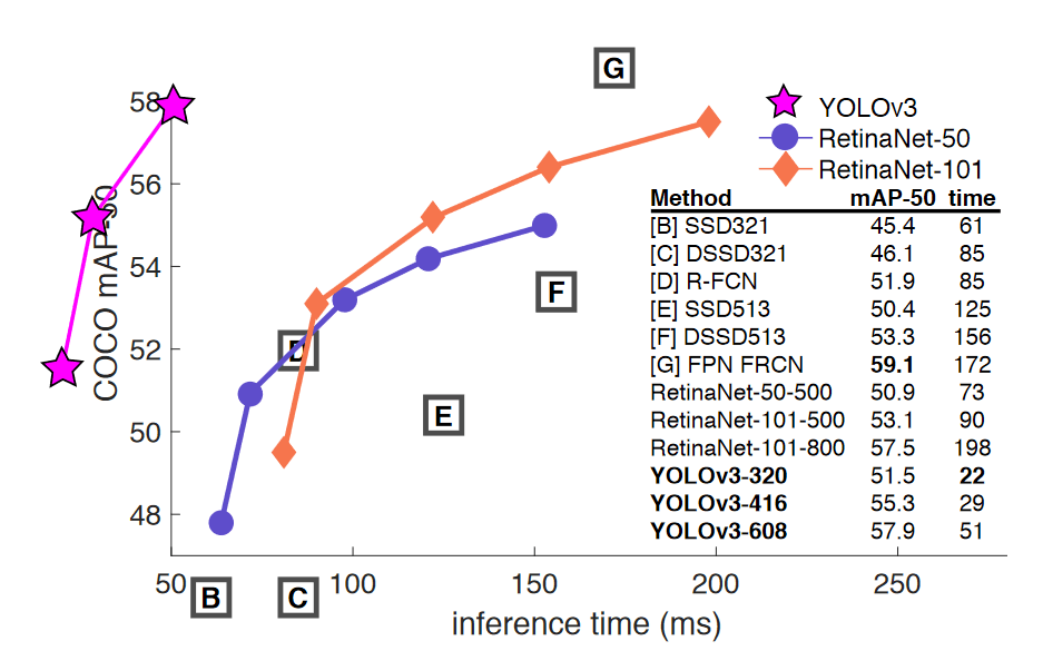
As a result, we get a statistical model that is not only able to process over 45 frames per second, but also gives a similar (though slightly lower) detection efficiency to definitely slower solutions.

YOLO fast object detection and classification – how does it work?
Traditional methods of detecting objects most often divide the entire process into several stages. For example, Faster R-CNN first uses a convolutional neural network to extract the desired features of the image (the so-called feature extraction). Then the output in the form of the feature map is an input to another neural network, the task of which is to suggest image regions where objects may be located. Such a network is called Region Proposal Network (RPN) and it is both a classifier (indicating the probability that a given region contains an object) and a regression model (describing a region of an image containing a potential object). The output of the RPN is passed to the third neural network, whose task is to predict classes of objects and bounding boxes. As you can see, it is quite a complicated, multi-stage process, that has to take quite a long time, at least compared to YOLO.
YOLO takes a completely different approach. First of all, it treats the detection and classification problems as a single regression problem. It does not divide the analysis into stages. Instead, a single convolutional neural network simultaneously predicts multiple bounding boxes and determines the class probabilities for each of the areas in which the object has been detected.
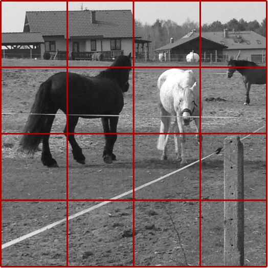
In the first step, YOLO puts a grid with the size of S x S on the image. For example, for S = 4, we get 16 cells, as in the image below.

For each cell YOLO predicts B objects. B is usually a small number, like 2. This means that we assume that in each cell YOLO will identify at most 2 objects. Of course, there may be more objects overlapping in the image. But when there are 3 or more overlapping objects in a given cell, they become very difficult to identify – especially when we consider the fact that S is usually greater than the one we used in our example (4), and therefore the applied grid has a higher granulation.
Thus, for each cell of the grid, YOLO predicts whether there are objects in it and for each of them the coordinates of the rectangle surrounding the object are determined (bounding box). This means that in the output vector we need to predict a place for B * 5 values. Why 5? This is because a bounding box is defined with 4 values: two coordinates of the center of the object (relative to the coordinates of the analyzed cell) and the width and height of the rectangle (as a fraction of the image size). In addition, there is a fifth value that logically determines whether or not there is an object in a given cell.
Finally, the class probabilities should be added to the output vector – for each object separately. For example, if we are going to predict C = 10 classes for a maximum of B = 2 objects in one grid cell, then the final output tensor will be: S x S x (B * (5 + C)). In our example: 4 x 4 x (2 * (5 + 10)) = 4 x 4 x 30.
So, we train the network and make predictions assuming a tensor on the output – hence it is easy to understand why the problem of object identification and classification was reduced by YOLO to the regression problem.
Two important points that may have caught your attention:
- If the algorithm identifies an object in a grid cell, is the bounding box somehow related to the grid cell? Yes and no. Yes, because this cell includes the center of the bounding box. No, because of course the actual surrounding rectangle will hardly ever coincide with the boundaries of the grid cell.
- Because the grid has the same number of rows and columns, the analyzed images must be square and have the size appropriate to the given YOLO implementation. If images are rectangular or do not correspond to the size expected by the network, many YOLO implementations resize the input images and transform them to aspect ratio = 1 (e.g. replenishing images with black padding).
YOLO – the architecture
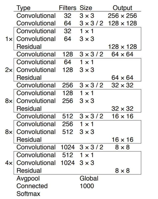
In the third version of the algorithm, the authors used the pretty extensive convolutional neural network with the architecture presented below. BTW: if you want to explore convolutional neural networks from scratch, there is a four-part tutorial on my blog.
The network has 53 convolutional layers, hence it was called Darknet-53.

YOLO in practice
Let’s see how YOLO behaves in practice. Installation instructions are available on the author’s website, but I was not able to successfully complete it on Windows 10. So I recommend switching to Linux or Mac right away. The following tips are for Ubuntu version 20.04.
To build the classifier you will need to be able to compile the code with gcc. If the compiler is not installed on the operating system (gcc – -version) then I suggest executing those three commands:
$ sudo apt update$ sudo apt install build-essential$ gcc --version
If the compiler version is displayed correctly, we can proceed with downloading and compiling Darknet:
$ git clone https://github.com/pjreddie/darknet$ cd darknet$ make
In the repository you will find the code, obviously, but the weights for the trained network have to be downloaded separately. The following command should be executed from the darknet directory and the file with network weights should also be saved there.
$ wget https://pjreddie.com/media/files/yolov3.weights
Depending on how much RAM we have (my Ubuntu only had 512MB RAM), the swapfile would have to be increased. I increased it to 2GB, but probably lower values will also be enough:
$ sudo fallocate -l 2G /swapfile$ sudo chmod 600 /swapfile$ sudo mkswap /swapfile$ sudo swapon /swapfile
At this point, we should be able to run a prediction for one of the sample photos in the data directory. Below is an example for the kite.jpg file. Note: it may be necessary to run prediction as a super user – hence sudo has been added:
$ sudo ./darknet detect cfg/yolov3.cfg yolov3.weights data/kite.jpg
The result is saved on the server in the predictions.jpg file. Here is the result for kites – input and output pictures combined:

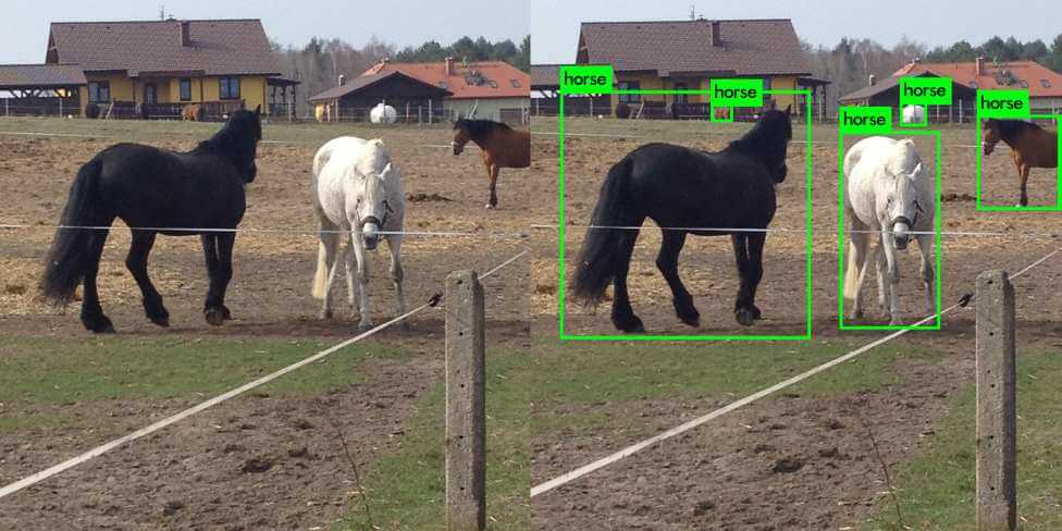
And below my photo with horses on the paddock:
$ sudo ./darknet detect cfg/yolov3.cfg yolov3.weights data/horses-square.jpg

As you can see, the horses were mostly located and correctly classified. Two of the three horses in the far background were not found, but it must be admitted that it would not be easy for the human eye either. A humorous accent is the qualification of the white gas tank as a horse, but it is also difficult to disagree that the tank in this perspective looks a bit like a horse’s rump from a distance. 😉
This mistake with the gas tank is paradoxically a confirmation of one of the strong features of YOLO – the algorithm looks at the image as a whole and infer contextually from the entire content of the image, not from a narrow fragment. YOLO has some problems with detecting small objects and will do worse with scenes with many overlapping objects, but overall it’s a brilliant architecture, written in C using CUDA, which makes it a very fast and effective tool for detecting and classifying objects in real time.
