k-nearest neighbors for handwriting recognition

If I had to indicate one algorithm in machine learning that is both very simple and highly effective, then my choice would be the k-nearest neighbors (KNN). What’s more, it’s not only simple and efficient, but it works well in surprisingly many areas of application. In this post I decided to check its effectiveness in the handwriting recognition. KNN may not be the first thought that comes to your mind when you try to recognize a handwriting, but as it turns out, using this method is not unreasonable. Intrigued just like me? I invite you to read further.

From this post you will learn:

• What are the most important features of KNN and in which classes of problems can it be used?
• How does the k-nearest neighbors algoritm work?
• How can you effectively classify handwriting using KNN?

What do you definitely need to know about k-nearest neighbors?

KNN is a very simple algorithm to understand and implement. At the same time, it offers surprisingly high efficiency in practical applications. Its simplicity, which is certainly its advantage, is also a feature that makes it sometimes unnecessarily overlooked when solving more complex problems. Interestingly, potential use of the algorithm is very wide. We can use it to provide both unsupervised and supervised learning, and the latter in both: regression and classification.

Reading the formal definition, it can be seen that KNN is characterized as a non-parametric and “lazy” algorithm. Non-parametric in this case does not mean that we do not have any hyperparameters here, as we have at least one parameter – the number of neighbors. It means only that this algorithm does not assume that we are dealing with a certain distribution of data. This is a very useful assumption, because in the real world the data we have available is often not easily linearly separable or does not reflect normal or any other type of distribution very well. Hence KNN can be useful, especially in cases where the relationship between the input data and the result is unusual or very complex, which means that classic methods such as linear or logistic regression may not be able to do the job.

Lazy in turn means that the algorithm does not build a model that generalizes a given problem in the learning phase. Learning, you can say, is deferred until the query about new data goes into the model. Two conclusions can be drawn from the above. Firstly, the testing / prediction phase will last longer than the “training” phase. Secondly, in most cases, the KNN will need all the data from the training set to be available during the prediction – this, in turn, imposes quite large requirements on the amount of memory for large datasets.

How does it work – a simple example.

The principle of the algorithm is best explained graphically and in two-dimensional space. Suppose we have a dataset described by two features (represented here by coordinates on a plane) and classified into two classes: circles and triangles.

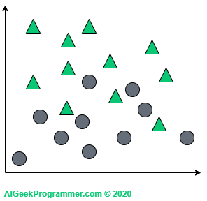
As you can see, this dataset is quite easily linearly separable, so it would probably be enough to use e.g. logistic regression for binary classification to get a great results, but for the purpose of explaining principles of the algorithm, this example will be perfect.

Suppose now that with such a dataset, we want to classify the new object (the red spot) as a triangle or circle:

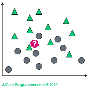
KNN works in such a way that it looks at “the closest area” of the new data and checks what class of objects are there and on the basis of this decides to describe it either as a triangle or as a circle. Okay, but what do we mean by “the closest area”? And here comes the k parameter, which determines how many closest neighbors we want to look at. If we look at one (which is a rather rare value of the k), it turns out that our new data is a triangle.

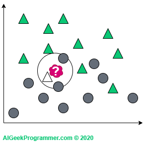
If we consider three neighbors, our red sample will change into a circle – just like in quantum physics 😉

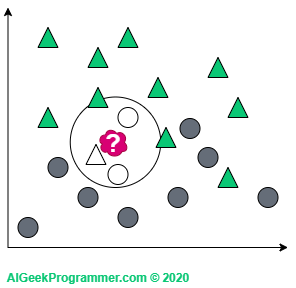
For k = 5 we are again dealing with the classification as a triangle, because in the immediate vicinity there are three triangles and two circles:

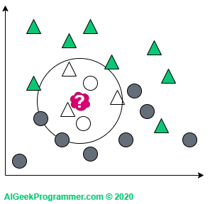
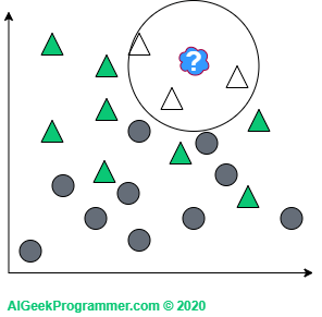
There are two points to note here. As you can see, I adopted odd k values only. This is justified because we will not come across a case in which a new data point is lying in the vicinity of two circles and two triangles. This does not mean that such k values are not used in practice. Simply for the above example, this would unnecessarily complicate our reasoning. Secondly, the new data appeared on the border between two classes. Therefore, it can be either a circle or a triangle, depending on the value of the parameter k. However, if a new object appears in a different, more “triangular” place, then regardless of the value of the parameter k, it will remain a triangle:

A slightly deeper look at the k-nearest neighbors algorithm

Although KNN is extremely simple, there are a few issues that are worth exploring, because as usual the devil is in the details.

How do we calculate the distance?

It seems quite obvious, but it is worth emphasizing at this point that the necessary condition to apply the k-nearest neighbors algorithm on a given dataset is the ability to calculate the distance between elements of this set. It does not have to be the Euclidean distance, but the inability to calculate the distance basically eliminates the KNN from the analysis of such a dataset.

In the two-dimensional Euclidean space, which we considered above, the distance can be calculated from the Pythagorean theorem. However, since we rarely analyze a dataset with only two features (i.e. two-dimensional), we should generalize the problem of distance to n-dimensional space. In that case the distance function can be defined by the following metric:

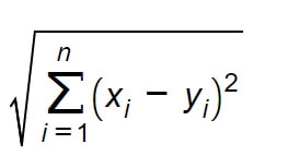
This is the most common way of calculating distance, but not the only one. The scikit-learn library, which we’ll use later, offers the possibility of using several different metrics, depending on the type of data and the type of task.

How to choose the value of k?

The number k is a hyperparameter and, as with other hyperparameters in machine learning, there is no rule or formula for determining its value. Therefore, it is best to determine it experimentally by assessing the accuracy of prediction for different k values. However, for large datasets it can be time consuming. So some tips could be helpful:

• Quite obviously, small k values will carry a greater risk of incorrect classification.
• On the other hand, large k values will give more reliable results, but will be much more computationally demanding. In addition, the k value set let’s say to 80, intuitively is in conflict with the idea of the nearest neighbors. After all, the point is to look at the immediate surroundings of the new data.
• In binary classification it is good to use odd values to avoid having to make a random selection in the event of an even distribution of votes,
• One of the commonly recommended k values to try is the square root of the number of elements in the training set. For example, if our training set has 1000 elements, then we should consider 32 as one of k values. For 50,000 it will be 224. Personally, I am not convinced by this method. I did not find its origin or scientific explanation (which does not mean that it does not exist). I believe that the values obtained in this way are too high.
• The method that seems more sensible to me is the 4th degree root of the amount of samples in the training set. For 500 samples it will be 5, for 1000 k = 6, for 50000 it is 15, and we would use k values above 30 for datasets with the amount of data exceeding one million.
• There are also methods that vote not on the basis of the k-nearest neighbors, but on the basis of votes collected from data within a specified radius from the examined point. Such a classifier – Radius Neighbors Classifier – is also offered by the scikit-learn library.
• However, it should be clearly stated that determining the optimal value of k is strongly dependent on the data and the problem under consideration, hence the above guidelines and formulas should be approached with caution and the best value should be determined experimentally.

What if the number of neighbors is the same in two or more classes?

This is an interesting case, because in such a situation it is just equally likely that the sample under study belongs to one of these two or more classes. The solution can be random selection or assigning weight to each of the nearest neighbors. The closer a neighbor is, the more important his weight is. The scikit-learn library offers a special parameter “weights”, which, set to ‘uniform’, assumes that each neighbor has the same weight, and set to ‘distance’ assigns weight to the neighbors inversely proportional to its distance from the examined data point.

And what about calculation efficiency?

With the increase in the amount of data (N) in the training set, the issue of the efficiency of calculations becomes more important. The least sophisticated approach is the use of ‘brute force’, i.e. calculating the distance between the examined point and all points in the training set. The cost of such a method increases exponentially, with the increase of N. For sets of several thousand samples and larger, the use of ‘brute force’ is basically impractical or unreasonable. Hence, more sophisticated methods are often used, based on tree structures, which boil down to the selection of points lying close to the examined data point. To put it simply: if the X point is very far from the Y point and the Z point is very close to the Y point, it can be assumed that the X and Z points are far apart and there is no need to calculate the distance for them. Scikit-learn implements two such structures: K-D Tree and Ball Tree. The library decides about their use based on the characteristics of the dataset, unless we intentionally impose one of the three abovementioned methods. This is described in detail in this section.

k-nearest neighbors in the handwriting classification

Okay, after a solid dose of theory let’s see how KNN deals with a practical issue. The scikit-learn library provides extensive tools for the k-nearest neighbors algorithm – it’s a shame not to use it. For the warm-up, we’ll take one of the toy datasets included in the scikit-learn – The Digits Dataset.

For the purposes of the following task, it’s best to create a new virtual conda environment. If you want to learn more about virtual environments, I invite you to read this post. On Windows, just run Anaconda prompt, go to the directory where you want to save the scripts and execute three simple commands:

conda create --name <name>
conda activate <name>
conda install numpy matplotlib scikit-learn jupyter keras

The environment configured in this way can be used by running jupyter notebook or by configuring a project based on this environment in your favorite IDE.

When performing the classification, we will have to use a number of components that must be imported at the beginning of the script. It is also a good test of whether the environment has been created and activated correctly:

from sklearn import datasets, neighbors
from sklearn.model_selection import train_test_split
from keras.datasets import mnist
import matplotlib.pyplot as plt
import numpy as np
from random import randint
import time

In the first step, we imported test datasets, including Digits, as well as the knn classifier. Later in the post, we will also need a function to divide the dataset into a training and test one, and a more advanced MNIST dataset, which can be downloaded from Keras. Matplotlib will provide us with graphical display of results, and of course we will use numpy for some operations on the dataset. Finally, two imports of helper functions related to random number generation and time measurement.

If all imports have been made correctly, we can proceed with further coding. To download the Digits dataset we’ll use a helper method offered by scikit-learn:

# load Digits data set divided into data X and labels y
X, y = datasets.load_digits(return_X_y=True)

# check data shapes - data is already flattened
print("X shape:", X.shape[0:])
print("y shape:", y.shape[0:])
>>> X shape: (1797, 64)
>>> y shape: (1797,)

The load_digits method, properly parameterized, returned the data to the variable X and the labels to the variable y. Let’s see a dozen or so randomly selected elements of the Digits dataset:

# let's see some random data samples.
pics_count = 16
digits = np.zeros((pics_count,8,8), dtype=int)
labels = np.zeros((pics_count,1), dtype=int)
for i in range(pics_count):
  idx = randint(0, X.shape[0]-1)
  # as data is flattened we need them to be reshaped to the original 2D shape
  digits[i] = X[idx].reshape(8,8)
  labels[i] = y[idx]

# then we print them all
fig = plt.figure()
fig.suptitle("A sample from the original dataset", fontsize=18)
for n, (digit, label) in enumerate(zip(digits, labels)):
  a = fig.add_subplot(4, 4, n + 1)
  plt.imshow(digit)
  a.set_title(label[0])
  a.axis('off')
fig.set_size_inches(fig.get_size_inches() * pics_count / 7)
plt.show()

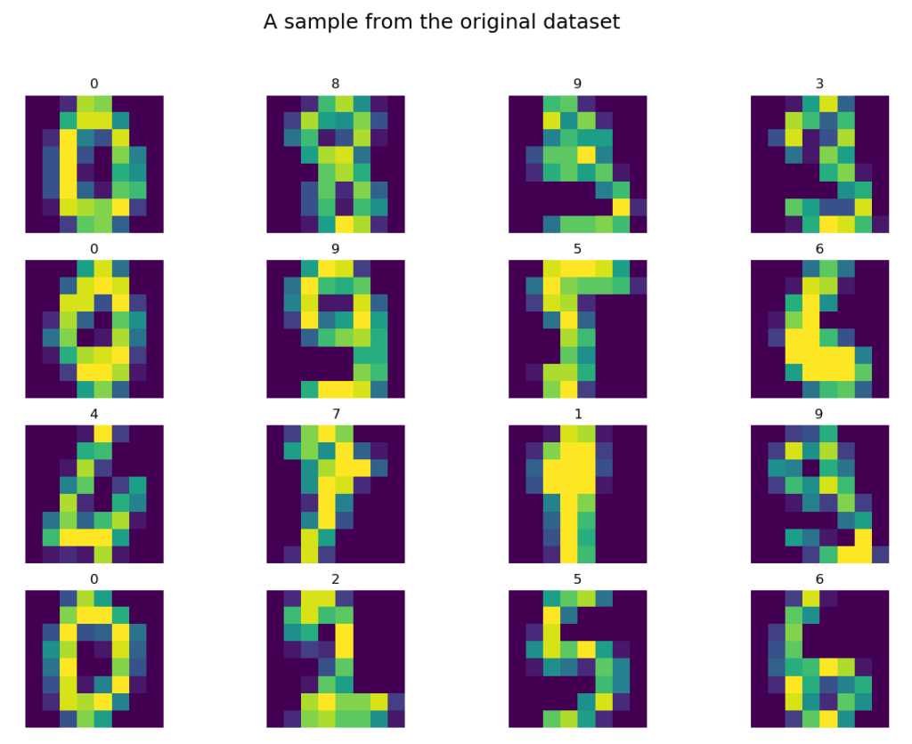
Well, it may not look like graphics in the World of Tanks, 😉 but most shapes are fairly simple to classify with a human eye. By the way, I wonder how many digits we would be able to quickly classify ourselves and whether this classification would be better than the results obtained by the algorithm. Hmmm…

We divide the dataset into training (70% of data) and test (30% of data) subsets to simulate the situation in which we receive new data – the new data will be the test set – and then we classify them based on the training set. Let’s remember that in the case of KNN we do not have classic learning phase, because the classifier is “lazy”:

# splitting into train and test data sets
X_train, X_test, y_train, y_test = train_test_split(X, y, test_size=0.3)

Let’s check the shapes of the variables obtained this way:

# checking shapes
print("X train shape:", X_train.shape[0:])
print("y train shape:", y_train.shape[0:])
print("X test shape:", X_test.shape[0:])
print("y test shape:", y_test.shape[0:])
>>> X train shape: (1257, 64)
>>> y train shape: (1257,)
>>> X test shape: (540, 64)
>>> y test shape: (540,)

Having the data loaded into the variables, we will define a classification function (lets_knn), which we’ll later also use for another dataset. The function accepts both: data and labels at the input, creates a classifier, processes the training set (knn.fit), and then performs prediction and determines the quality of the classification (accuracy). Finally, we display the results of the classification, and also identify which data was classified incorrectly (wrong_pred), with what label (wrong_labels) and what is the correct one (correct_labels). The function also accepts, as parameters, the number of neighbors, the method for determining distance weights, and the parameter specifying whether to present incorrect predictions in a graphic form:

def lets_knn(X_train, y_train, X_test, y_test, n_neighbors=3, weights='uniform', print_wrong_pred=False):
    t0 = time.time()
    # creating and training knn classifier
    knn = neighbors.KNeighborsClassifier(n_neighbors=n_neighbors, weights=weights)
    knn.fit(X_train, y_train)
    t1 = time.time()

    # predicting classes and comparing them with actual labels
    pred = knn.predict(X_test)
    t2 = time.time()
    # calculating accuracy
    accuracy = round(np.mean(pred == y_test)*100, 1)

    print("Accuracy of", weights ,"KNN with", n_neighbors, "neighbors:", accuracy,"%. Fit in",
          round(t1 - t0, 1), "s. Prediction in", round(t2 - t1, 1), "s")

    # selecting wrong predictions with correct and wrong labels
    wrong_pred = X_test[(pred != y_test)]
    correct_labels = y_test[(pred != y_test)]
    wrong_labels = pred[(pred != y_test)]

    if print_wrong_pred:
        # the we print first 16 of them
        fig = plt.figure()
        fig.suptitle("Incorrect predictions", fontsize=18)
        # in order to print different sized photos, we need to determine to what shape we want to reshape
        size = int(np.sqrt(X_train.shape[1]))
        for n, (digit, wrong_label, correct_label) in enumerate(zip(wrong_pred, wrong_labels, correct_labels)):
            a = fig.add_subplot(4, 4, n + 1)
            plt.imshow(digit.reshape(size,size))
            a.set_title("Correct: " + str(correct_label) + ". Predicted: " + str(wrong_label))
            a.axis('off')
            if n == 15:
                break
        fig.set_size_inches(fig.get_size_inches() * pics_count / 7)
        plt.show()

Let’s use the above function to make predictions for the Digits dataset:

lets_knn(X_train, y_train, X_test, y_test, 5, 'uniform', print_wrong_pred=True)
>>> Accuracy of uniform KNN with 5 neighbors: 98.0 %. Fit in 0.0 s. Prediction in 0.1 s

The function was called for k = 5 neighbors, with uniform weights (‘uniform’) for each distance and obtained a decent accuracy of 98%.

Let’s look at the data that was classified incorrectly:

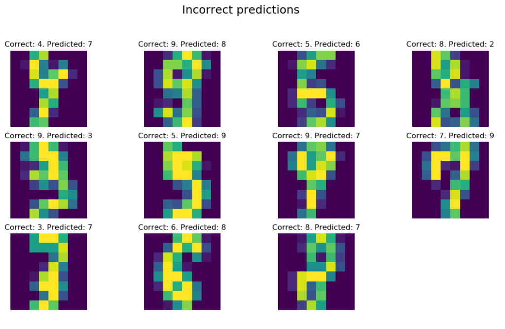
Well, I don’t know. 😉 I would disagree with some “correct” labels or at least I would have to think about the correct answer a little bit longer. As you can see, KNN did its job pretty well, as the above are all incorrect predictions on 540 test samples.

Let’s check now how our classifier will deal with a much larger and more demanding MNIST dataset . If anyone wanted to know a little more about the MNIST dataset, I wrote about it at the very beginning of the post about the handwriting classification. The simplest way to load MNIST dataset is to use the loader from the Keras library:

# now let's play with MNIST data set
(X_train, y_train), (X_test, y_test) = mnist.load_data()
# checking initial shapes
print("X train initial shape:", X_train.shape[0:])
print("y train initial shape:", y_train.shape[0:])
print("X test initial shape:", X_test.shape[0:])
print("y test initial shape:", y_test.shape[0:])
>>> X train initial shape: (60000, 28, 28)
>>> y train initial shape: (60000,)
>>> X test initial shape: (10000, 28, 28)
>>> y test initial shape: (10000,)

As you can see, we have 60000 samples in the training set and 10000 in the test set. In addition, each element from the set is a 28 x 28 image, which compared to the Digits dataset, with its 8 x 8, gives 12 times deeper data dimension. Classification on such an amount of data will take a lot of time. As discussed above, k-nearest neighbors algorithm is a lazy classifier, which means that most calculations take place in the prediction phase. Therefore, it is worth limiting the amount of data in the test set, which should significantly speed up the whole process. Of course, if you have a sufficiently strong computing environment or you have a lot of time, you can experiment with larger values. Unfortunately, the scikit-learn library does not offer GPU support:

# Reducing the size of testing data set, as it's the most time-consuming
X_train = X_train[:60000]
y_train = y_train[:60000]
X_test = X_test[:1000]
y_test = y_test[:1000]

We have loaded data as two-dimensional: 28 x 28. Machine learning expects a vector, hence we must flatten it:

# reshaping
X_train = X_train.reshape((-1, 28*28))
X_test = X_test.reshape((-1, 28*28))

# checking shapes
print("X train shape:", X_train.shape[0:])
print("y train shape:", y_train.shape[0:])
print("X test shape:", X_test.shape[0:])
print("y test shape:", y_test.shape[0:])
>>> X train shape: (60000, 784)
>>> y train shape: (60000,)
>>> X test shape: (1000, 784)
>>> y test shape: (1000,)

We are now ready to run our classifier. To make it more interesting, we’ll run it for different k values and for two ways of determining the weights of the nearest neighbors:

# lets run it with different parameters to check which one is the best
for weights in ['uniform', 'distance']:
  for n in range(1,11):
     lets_knn(X_train, y_train, X_test, y_test, n_neighbors=n, weights=weights, print_wrong_pred=True)

>>> Accuracy of uniform KNN with 1 neighbors: 96.2 %. Fit in 49.2 s. Prediction in 63.5 s
>>> Accuracy of uniform KNN with 2 neighbors: 94.8 %. Fit in 50.4 s. Prediction in 61.4 s
>>> Accuracy of uniform KNN with 3 neighbors: 96.2 %. Fit in 47.6 s. Prediction in 61.4 s
>>> Accuracy of uniform KNN with 4 neighbors: 96.4 %. Fit in 46.1 s. Prediction in 61.0 s
>>> Accuracy of uniform KNN with 5 neighbors: 96.1 %. Fit in 47.2 s. Prediction in 60.7 s
>>> Accuracy of uniform KNN with 6 neighbors: 95.9 %. Fit in 46.1 s. Prediction in 60.7 s
>>> Accuracy of uniform KNN with 7 neighbors: 96.2 %. Fit in 46.4 s. Prediction in 60.8 s
>>> Accuracy of uniform KNN with 8 neighbors: 95.8 %. Fit in 47.5 s. Prediction in 60.8 s
>>> Accuracy of uniform KNN with 9 neighbors: 95.2 %. Fit in 46.3 s. Prediction in 61.8 s
>>> Accuracy of uniform KNN with 10 neighbors: 95.4 %. Fit in 50.8 s. Prediction in 62.8 s
>>> Accuracy of distance KNN with 1 neighbors: 96.2 %. Fit in 48.7 s. Prediction in 63.1 s
>>> Accuracy of distance KNN with 2 neighbors: 96.2 %. Fit in 53.2 s. Prediction in 63.5 s
>>> Accuracy of distance KNN with 3 neighbors: 96.5 %. Fit in 51.5 s. Prediction in 63.0 s
>>> Accuracy of distance KNN with 4 neighbors: 96.4 %. Fit in 50.3 s. Prediction in 60.5 s
>>> Accuracy of distance KNN with 5 neighbors: 96.4 %. Fit in 46.0 s. Prediction in 60.4 s
>>> Accuracy of distance KNN with 6 neighbors: 96.5 %. Fit in 48.5 s. Prediction in 61.5 s
>>> Accuracy of distance KNN with 7 neighbors: 96.4 %. Fit in 48.6 s. Prediction in 61.5 s
>>> Accuracy of distance KNN with 8 neighbors: 96.4 %. Fit in 48.3 s. Prediction in 61.5 s
>>> Accuracy of distance KNN with 9 neighbors: 95.7 %. Fit in 48.1 s. Prediction in 61.6 s
>>> Accuracy of distance KNN with 10 neighbors: 95.7 %. Fit in 48.4 s. Prediction in 61.5 s

The results are very similar for all configurations. I did not paste results for larger k, but raising the parameter value, even to 20, does not change the situation. It seems that for the MNIST dataset slightly better results are given by ‘distance’ weighted measurement – for which we recorded two best results of the classification: 96.5% for k = 3 and the same accuracy for k = 6. It is also worth paying attention to the much longer classification times than in the case of the Digits dataset. The “training” phase lasts about 49s, and the prediction phase about 61s.

Finally, let’s take a look at some examples of misclassification:

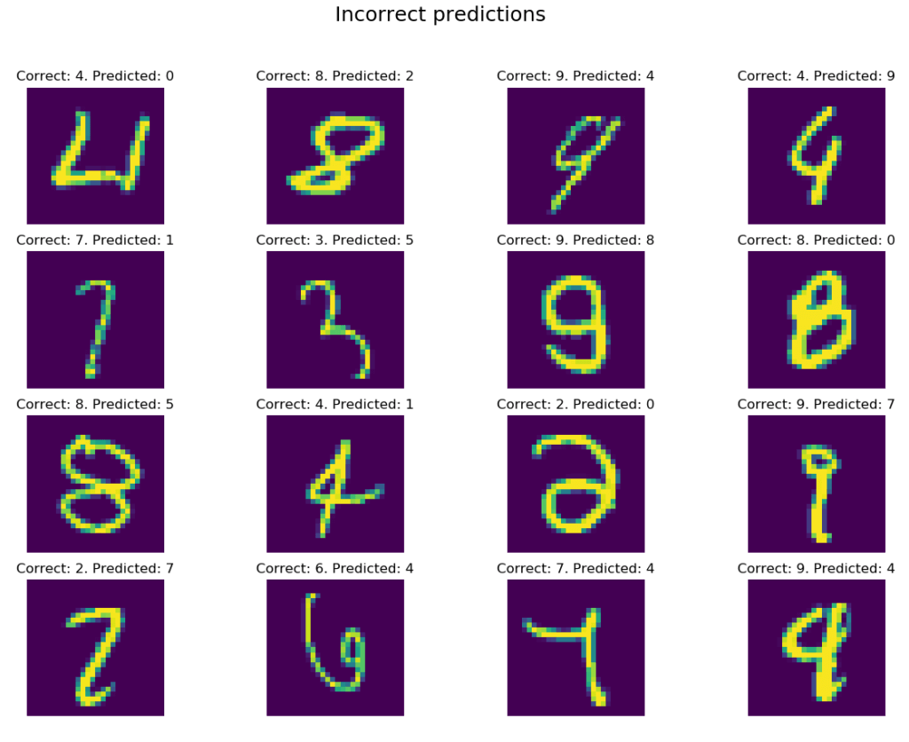
With the exception of a few items: (row 1, column 3), (2, 1), (3, 3), (4, 3) and (4, 4), errors are slightly more obvious than in the case of the Digits dataset. Nevertheless, a classification of 96.5% for such a simple algorithm can make a good impression.

In this post I have introduced you to the theoretical foundations behind the k-nearest neighbors algorithm. We also used the algorithm in practice, solving two classification problems. k-nearest neighbors, despite its simplicity and ease of use, gives very good results on a number of issues and I hope that I encouraged you to use this method more often.

---