Convolutional neural network 4: data augmentation

In the previous three parts of the tutorial, we learned about convolutional networks in detail. We looked at the convolution operation, the convolutional network architecture, and the problem of overfitting. In the classification of the CIFAR-10 dataset we achieved 81% on the test set. To go further we would have to change the architecture of our network, experiment with hyperparameters or get more data. I leave the first two solutions for you 😉 to experiment with, and in this part of the tutorial I want to feed our network with more data. I will use the so-called data augmentation, i.e. the artificial generation of large amounts of new data.

In the fourth part of the tutorial you will learn:

• What is data augmentation?
• How to use the data generator from the Keras library?
• How to artificially generate new data for the CIFAR-10 set?
• And how well will our model do on the set of artificially generated (augmented) data?

What is data augmentation?

As I mentioned in the previous part of the tutorial, if we are dealing with a closed data set, i.e. one that cannot be significantly enlarged or enlarged is very expensive, we can reach for the so-called data augmentation. This is a particularly valuable technique for image analysis. Why? Because the images are susceptible to minor modifications, which will be a new data for the algorithm, although they will still be basically the same for the human eye. Moreover, such “minor modifications” occur in the real world. Standing in front of the car, we can look at it centrally or slightly from the side. It will still be the same vehicle and it will definitely be a car for our brain. For the algorithm, looking at the object from a different perspective is valuable information that allows to better generalize the training process.

What can we actually do with the image we want to artificially process? In theory, we have infinitely many solutions: we can slightly rotate the image, in any direction, at any angle. Move left, right, up and down. Change its colors or make other more or less subtle changes that will give the model tons of new data. In practice, a collection of tens of thousands of images can become a collection with millions of elements. This is a field where the possibilities are really great. As a curiosity: technologies related to autonomous vehicles are also trained on artificially generated data sets, e.g. using realistic game environments such as GTA.

Generating data with the Keras library

The Keras library offers a set of helpful tools for generating data. Let’s try to process the previously seen picture of the building in Crete with this generator. First, we make the necessary imports and define a function that will load the image from the file and convert it to the numpy table:

import numpy as np
from PIL import Image
import matplotlib.pyplot as plt
%matplotlib inline

def convert_image(file):
  return np.array(Image.open(file))

We load a picture that you can download here, display the shape of the numpy table and the picture itself:

image = convert_image(r'<<path-to-the-file-on-disc>>\house-small.jpg')
image.shape
>>> (302, 403, 3)

plt.imshow(image)

To generate data we will use the flow (x, y) method from the ImageDataGenerator class. To be able to use it correctly, we have to import the class – that’s pretty obvious, but also adapt the data accordingly. The method expects the tensor x, in which the first position will be the index. In our case, there will be only one element, but the method still requires an index. Inputs y are labels that we don’t need for this simple experiment, but we must provide them. Hence:

from tensorflow.keras.preprocessing.image import ImageDataGenerator

x = np.expand_dims(image, 0)
x.shape
>>> (1, 302, 403, 3)

y = np.asarray(['any-label'])

Then we create the generator object and we pass the appropriate parameters. In the specification there are tons of them available, below are only few examples:

datagen = ImageDataGenerator(
  width_shift_range=0.2, # shift along the x axis
  height_shift_range=0.2, # shift along the y axis
  rotation_range=20,
  horizontal_flip=True,
  vertical_flip = True,
  rescale=1./255,
  shear_range=0.25,
  zoom_range=0.25,
)

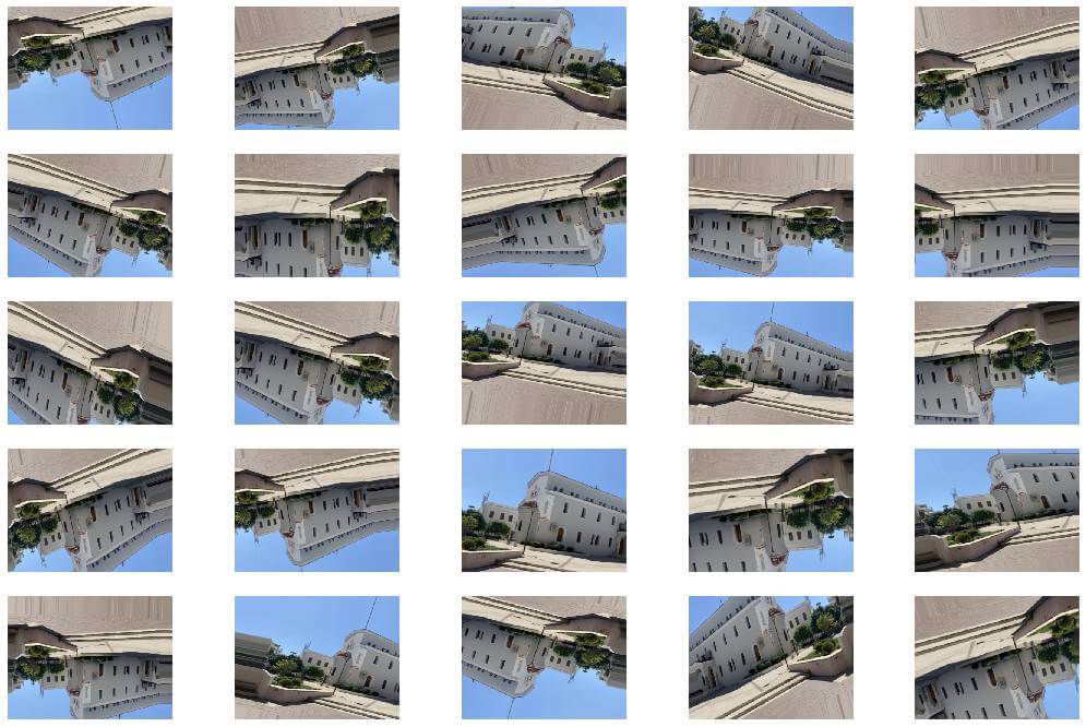
Now we just call the flow (x, y) method, passing the prepared data to it and receiving and displaying the generated images.

figure = plt.figure()
i = 0
for x_batch, y_batch in datagen.flow(x, y):
  a = figure.add_subplot(5, 5, i + 1)
  plt.imshow(np.squeeze(x_batch))
  a.axis('off')
  if i == 24: break
  i += 1
figure.set_size_inches(np.array(figure.get_size_inches()) * 3)
plt.show()

The result? Literally a bit upside down 😉 and a little “exaggerated”, because some parameters are set to high values. But it well reflects the capabilities of the generator. You can experiment with the settings yourself.

Data augmentation on CIFAR-10

Armed with a generator, we can once again approach the classification of the CIFAR-10 dataset. Most of the code has already been discussed in the previous parts of the tutorial, so I will only provide it here for consistency and clarity. At the beginning we make the necessary imports, load the dataset and build a model:

import numpy as np

%tensorflow_version 2.x
import tensorflow

import matplotlib.pyplot as plt
%matplotlib inline

After preparing and successfully compiling the model, we define the generator. We assume that the data will be rotated by 10 degrees, we allow horizontal flip, but not vertical in order not to artificially put things upside down. The generator will also move the images vertically and horizontally by 10%. Small zoom and shear are also allowed. Let’s remember that the images are small and major modifications can make the image difficult to recognize even for a person:

We also need one-hot encoding for training and test labels. We set the size of the batch and the generator is basically ready to use:

y_train = to_categorical(y_train)
y_test = to_categorical(y_test)

batch_size = 64
train_generator = datagen.flow(x_train, y_train, batch_size=batch_size)

The above generator will be the source of data for the training process. But what about the validation set that will allow us to track progress? Well, we need to define a separate generator. However, this one will not modify the source images in any way:

datagen_valid = ImageDataGenerator(
  rescale = 1. / 255,
)

x_valid = x_train[:100*batch_size]
y_valid = y_train[:100*batch_size]

x_valid.shape[0]
>>>6400

valid_steps = x_valid.shape[0] // batch_size
validation_generator = datagen_valid.flow(x_valid, y_valid, batch_size=batch_size)

As you can see above, the dataset that the training process will use for validation will be 100 times batch size. We also need to calculate the number of validation steps – these data will be needed to start the training.

history = model.fit_generator(
  train_generator,
  steps_per_epoch=len(x_train) // batch_size,
  epochs=120,
  validation_data=validation_generator,
  validation_freq=1,
  validation_steps=valid_steps,
  verbose=2
)

Note that we are not using the fit() method as before, but the fit_generator() method, which accepts a training data generator and (optionally) a validation data generator. With so much data, we will teach 120 instead of 80 epochs, hoping to avoid overfitting.

>>> Epoch 1/120
>>> Epoch 1/120
>>> 781/781 - 49s - loss: 1.8050 - acc: 0.3331 - val_loss: 1.5368 - val_acc: 0.4581
>>> Epoch 2/120
>>> Epoch 1/120
>>> 781/781 - 41s - loss: 1.3230 - acc: 0.5249 - val_loss: 1.1828 - val_acc: 0.5916
>>> Epoch 3/120

(...)

>>> 781/781 - 39s - loss: 0.1679 - acc: 0.9473 - val_loss: 0.1484 - val_acc: 0.9463
>>> Epoch 119/120
>>> Epoch 1/120
>>> 781/781 - 38s - loss: 0.1708 - acc: 0.9466 - val_loss: 0.1538 - val_acc: 0.9538
>>> Epoch 120/120
>>> Epoch 1/120
>>> 781/781 - 39s - loss: 0.1681 - acc: 0.9486 - val_loss: 0.1379 - val_acc: 0.9534

We obtained accuracy of 95% for both sets. This can also be seen in the chart below:

print(history.history.keys())
>>> dict_keys(['loss', 'acc', 'val_loss', 'val_acc'])

plt.plot(history.history['acc'])
plt.plot(history.history['val_acc'])
plt.title('Model accuracy')
plt.ylabel('Accuracy')
plt.xlabel('Epoch')
plt.legend(['Train', 'Valid'], loc='upper left')
plt.show()

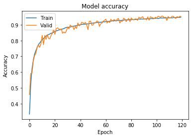
Due to the lack of overfitting, we could theoretically further increase the number of epochs.

Let’s check how the trained model will cope with the test dataset that it has not yet seen.

x_final_test = x_test / 255.0
eval = model.evaluate(x_final_test, y_test)
>>> 10000/10000 [==============================] - 3s 314us/sample - loss: 0.5128 - acc: 0.8687

We achieved accuracy of 87%, 6% more than the model version without a data generator.

Most importantly, however, the model is eager to continue learning, without compromising accuracy on the validation and test sets.

---

This is the last post in this tutorial. I hope that I was able to bring some interesting topics related to convolutional neural networks. If you liked the above post and the entire tutorial, please share it with people who may be interested in the subject of machine learning.